
Computing Optimal Hypertree Decompositions with SAT
Proceedings of the Thirtieth International Joint Conference on Artificial Intelligence. Main Track. Pages 1418-1424.
https://doi.org/10.24963/ijcai.2021/196
Keywords
- Constraints and SAT: Satisfiability Modulo Theories
- Constraints and SAT: Constraints: Modeling, Solvers, Applications
- Constraints and SAT: Constraint Satisfaction
Abstract
Hypertree width is a prominent hypergraph invariant with many
algorithmic applications in constraint satisfaction and
databases. We propose a novel characterization for hypertree width
in terms of linear elimination orderings. We utilize this
characterization to generate a new SAT encoding that we evaluate on
an extensive set of benchmark instances. We compare it to
state-of-the-art exact methods for computing optimal hypertree
width. Our results show that the encoding based on the new
characterization is not only significantly more compact than known
encodings but also outperforms the other methods.
- [Bachoore and Bodlaender, 2006] Emgad H. Bachoore and Hans L. Bodlaender. A branch and bound algorithm for exact, upper, and lower bounds on treewidth. Technical report, Department of Information and Computing Sci- ences,Utrecht University, 2006.
- [Bailleux and Boufkhad, 2003] Olivier Bailleux and Yacine Boufkhad. Efficient CNF encoding of boolean cardinal- ity constraints. In Francesca Rossi, editor, Proc. CP '03, volume 2833 of Lecture Notes in Computer Science, pages 108-122. Springer, 2003.
- [Bannach et al., 2017] Max Bannach, Sebastian Berndt, and Thorsten Ehlers. Jdrasil: A modular library for computing tree decompositions. In Costas S. Iliopoulos, Solon P. Pissis, Simon J. Puglisi, and Rajeev Raman, editors, Proc. SEA '17, volume 75 of LIPIcs, pages 28:1-28:21. Schloss Dagstuhl - Leibniz-Zentrum fuer Informatik, 2017.
- [Benedikt et al., 2017] Michael Benedikt, George Konstan- tinidis, Giansalvatore Mecca, Boris Motik, Paolo Papotti, Donatello Santoro, and Efthymia Tsamoura. Benchmark- ing the chase. In Proc. PODS '17, page 37-52, New York, NY, USA, 2017. Association for Computing Machinery.
- [Berg et al., 2017] Jeremias Berg, Neha Lodha, Matti Järvisalo, and Stefan Szeider. MaxSAT benchmarks based on determining generalized hypertree-width. In MaxSAT Evaluation 2017, page 22. Department of Computer Sci- ence, University of Helsinki, 2017.
- [Bodlaender, 2005] Hans L. Bodlaender. Discovering treewidth. In Proc. SOFSEM '05, volume 3381 of LNCS, pages 1-16. Springer Verlag, 2005.
- [Bonifati et al., 2017] Angela Bonifati, Wim Martens, and Thomas Timm. An analytical study of large sparql query logs. Proc. VLDB Endowment, 11(2):149-161, October 2017.
- [Bonifati et al., 2019] Angela Bonifati, Wim Martens, and Thomas Timm. Navigating the maze of wikidata query logs. In Proc. WWW '19, page 127-138, New York, NY, USA, 2019. Association for Computing Machinery.
- [Dzulfikar et al., 2020] Muhammad Ayaz Dzulfikar, Jo- hannes Klaus Fichte, and Markus Hecher. The PACE 2019 parameterized algorithms and computational experiments challenge: The fourth iteration. In Proc. IPEC '19, 2020.
- [Fichte et al., 2018] Johannes Klaus Fichte, Markus Hecher, Neha Lodha, and Stefan Szeider. An SMT approach to fractional hypertree width. In Proc. CP '18, volume 11008 of LNCS, pages 109-127. Springer Verlag, 2018.
- [Fischl et al., 2018] Wolfgang Fischl, Georg Gottlob, and Reinhard Pichler. General and Fractional Hypertree De- compositions. In Proc. SIGMOD/PODS '18, pages 17-32, New York, New York, USA, 2018. ACM Press.
- [Fischl et al., 2019] Wolfgang Fischl, Georg Gottlob, Da- vide Mario Longo, and Reinhard Pichler. Hyperbench: A benchmark and tool for hypergraphs and empirical find- ings. In Proc. PODS '19, pages 464-480. Assoc. Comput. Mach., New York, 2019.
- [Gogate and Dechter, 2004] Vibhav Gogate and Rina Dechter. A complete anytime algorithm for treewidth. In Proc. UAI '04), pages 201-208, Arlington, Virginia, 2004. AUAI Press.
- [Gottlob and Samer, 2009] Georg Gottlob and Marko Samer. A backtracking-based algorithm for hypertree decompo- sition. J. Exp. Algorithmics, 13:1:1.1-1:1.19, February 2009.
- [Gottlob et al., 2002] Georg Gottlob, Nicola Leone, and Francesco Scarcello. Hypertree decompositions and tractable queries. J. of Computer and System Sciences, 64(3):579-627, 2002.
- [Gottlob et al., 2003] Georg Gottlob, Nicola Leone, and Francesco Scarcello. Robbers, marshals, and guards: game theoretic and logical characterizations of hypertree width. J. of Computer and System Sciences, 66(4):775-808, 2003.
- [Gottlob et al., 2005] Georg Gottlob, Martin Grohe, Nysret Musliu, Marko Samer, and Francesco Scarcello. Hypertree decompositions: Structure, algorithms, and applications. In Dieter Kratsch, editor, Proc. WG '05), volume 3787 of LNCS, pages 1-15. Springer Verlag, 2005.
- [Gottlob et al., 2014] Georg Gottlob, Gianluigi Greco, and Francesco Scarcello. Treewidth and hypertree width. In Tractability: Practical Approaches to Hard Problems, pages 3-38. Cambridge University Press, 2014.
- [Grohe and Marx, 2014] Martin Grohe and Dániel Marx. Constraint solving via fractional edge covers. ACM Trans- actions on Algorithms, 11(1):Art. 4, 20, 2014.
- [Ignatiev et al., 2018] Alexey Ignatiev, Antonio Morgado, and Joao Marques-Silva. PySAT: A Python toolkit for prototyping with SAT oracles. In Proc. SAT '18, pages 428-437, 2018.
- [Korhonen et al., 2019] Tuukka Korhonen, Jeremias Berg, and Matti Järvisalo. Solving graph problems via poten- tial maximal cliques: An experimental evaluation of the Bouchitté-Todinca algorithm. J. Exp. Algorithmics, 24(1), February 2019.
- [Lodha et al., 2017] Neha Lodha, Sebastian Ordyniak, and Stefan Szeider. SAT-encodings for special treewidth and pathwidth. In Proc. SAT '17, volume 10491 of LNCS, pages 429-445. Springer Verlag, 2017.
- [Martins et al., 2014] Ruben Martins, Saurabh Joshi, Vasco Manquinho, and Inês Lynce. Incremental cardinality con- straints for maxsat. In Proc. CP '14, pages 531-548, Cham, 2014. Springer International Publishing.
- [Pottinger and Halevy, 2001] Rachel Pottinger and Alon Halevy. Minicon: A scalable algorithm for answering queries using views. The VLDB Journal, 10(2-3):182-198, September 2001.
- [Samer and Veith, 2009] Marko Samer and Helmut Veith. En- coding treewidth into SAT. In Proc. SAT '09, volume 5584 of LNCS, pages 45-50. Springer Verlag, 2009.
- [Schidler and Szeider, 2020] André Schidler and Stefan Szei- der. Computing optimal hypertree decompositions. In Proc. ALENEX '20, pages 1-11. SIAM, 2020.
References were extracted automatically from the PDF and may contain errors.
Full text extracted automatically from the PDF; figures, tables and equations may differ. The PDF is the version of record.
1 Introduction
Hypertree width is a popular hypergraph invariant which was introduced by Gottlob et al. [2002]. Hypertree width is of fundamental nature, as underpinned by the existence of combinatorial, game-theoretic, as well as logical characterisations [Gottlob et al., 2003]. In their original paper, Gottlob et al. [2002] showed that critical NP-hard problems arising in databases and constraint satisfaction are polynomial-time tractable for instances whose associated hypergraph has bounded hypertree width. The hypergraph invariant has found many further applications, including Projected Solution Counting, Solution Enumeration (with polynomial delay), Constraint Optimization, and Combinatorial Auctions (see, for example, the survey article [Gottlob et al., 2014]).
Key to these tractability results is the fact that for any fixed constant bound W, one can decide in polynomial time 1 whether a given hypergraph has hypertree width up to W, and in the positive case compute a witnessing hypertree decomposition of width W. Thus, the problem of recognizing hypergraphs of hypertree width W is in XP, when parameterized by W. However, the problem is known to be W[2]-hard [Gottlob et al., 2005] and hence unlikely to be fixed-parameter tractable. The original XP-algorithm by Gottlob et al. [2002] was later improved by Gottlob and Samer [2009], and their implementation of the algorithm (det-k-decomp) represented for several years the state-of-the-art for practically computing optimal hypertree decompositions. Only recently, Schidler and Szeider [2020] proposed a new algorithmic approach for computing optimal hypertree decompositions, which outperformed the known combinatorial algorithm on many instances 2 . This new approach is based on an encoding of the decomposition problem as a propositional satisfiability problem (SAT), which is then solved by a SAT-solver (more precisely, a so-called SAT Modulo Theory solver). The encoding, however, is complicated and produces large SAT instances. Therefore, Schidler and Szeider's approach utilizes a portfolio of algorithms, where several heuristics are tried first, and only when they fail, the expensive SAT encoding is used. The reason for the relative inefficiency of the encoding is the fact that in contrast to other width measures like treewidth, no characterisation of hypertree width is known that is based on linear elimination orderings. Such characterisations provide the basis for highly efficient algorithms for the corresponding decomposition problems, for example SAT/SMT encodings [Fichte et al., 2018; Samer and Veith, 2009] and Branch & Bound algorithms [Bachoore and Bodlaender, 2006; Gogate and Dechter, 2004].
1 The recognition problem is complete for the complexity class LOGCFL, which is contained in AC1 and hence highly parallelizable.
Contribution. In this paper, we give a first characterisation of hypertree width in terms of linear elimination orderings (LEO) and utilize this characterisation for a new SAT encoding. The encoding is not only significantly more compact than the above mentioned encoding used in Schidler and Szeider's portfolio, but also highly efficient. Although we tested the new LEO characterisation of hypertree width only in the SAT encoding, we believe that this characterisation will be of interest in other contexts. For instance, we expect that one can build new Branch & Bound algorithms for hypertree width on top of the LEO characterisation.
Our characterisation is based on a closer analysis of the combinatorics within a hypertree decomposition. The main ingredient is the observation that we do not need to have an explicit representation of a decomposition tree (as in the previous encoding), but it suffices to work with an ancestry relation, which is a direct by-product of the elimination ordering. Another important ingredient is an efficient way of dealing with "accumulating hyperedges" (see Section 3), an issue that arises when using a standard elimination ordering approach. We resolve this issue with the concept of arc-paths, which can be efficiently encoded. This is contrast to the previous encoding [Schidler and Szeider, 2020] which entails an explicit representation of a decomposition tree and an elimination DAG together with an equivalence relation on the vertices.
2 Hypertree width was subject of PACE 2019 [Dzulfikar et al., 2020], where Schidler and Szeider's solver won the exact track, tailed by a new implementation of Gottlob and Samer's algorithm.
We implemented the new LEO-based encoding and tested it on an extensive set of benchmark instances (Hyperbench), consisting of real-world hypergraphs from various application domains, with a number of vertices and hyperedges ranging up to 2900. We tested two variants, one where the cardinality constraints are encoded using binary counters (plain SAT) and one where the cardinality constraints are encoded by arithmetic constraints that are dealt with by the theory component of a SAT Modulo Theory solver (SMT). We compared our approach with Schidler and Szeider's portfolio [2020] as well as Gottlob and Samer's combinatorial XP-algorithm det-kdecomp [2009].
The results are highly encouraging and show that the LEO-based encoding outperforms all the other mentioned approaches.
2 Preliminaries
A hypergraph is a pair H = (V, E), consisting of a set V (H) of vertices and a set E(H) of hyperedges, each hyperedge is a subset of V (H). The primal graph (or 2-section) of a hypergraph H = (V, E) is the graph P(H) = (V (H), E(P(H))) with E(P(H)) = { {u, v} | u ̸= v, there is some e ∈ E such that {u, v} ⊆ e }. Consider a hypergraph H = (V, E) and a set S ⊆ V . An edge cover of S (with respect to H) is a set F ⊆ E such that for every v ∈ S there is some e ∈ F with v ∈ e. The size of an edge cover is its cardinality. Given an edge cover F , we use the shorthand ⋃ F := ⋃e∈F e.
A tree decomposition of a hypergraph H = (V, E) is a pair T = (T, χ) where T = (V (T),E(T)) is a tree and χ is a mapping that assigns to each t ∈ V (T) a set χ(t) ⊆ V (called the bag at t) such that the following properties hold:
- T1 for each v ∈ V there is some t ∈ V (T) with v ∈ χ(t) ("v is covered by t"),
- T2 for each e ∈ E there is some t ∈ V (T) with e ⊆ χ(t) ("e is covered by t"),
- T3 for any three t, t′ , t′′ ∈ V (T) where t′ lies on the path between t and t′′ , we have χ(t) ∩ χ(t′′ ) ⊆ χ(t′ ) ("bags containing the same vertex are connected").
A hypertree decomposition [Gottlob et al., 2002] of H is a triple D = (T, χD, λD) where (T, χD) is a tree decomposition of H, and λD is a mapping that assigns each t ∈ V (T ) an edge cover λD(t) ⊆ E(H) of χD(t). The width of D is the size of the largest edge cover in λD. Moreover, the tree T is rooted and satisfies in addition to T1-T3 also a certain Special Condition (T4). To formulate the Special Condition, we call a vertex v to be omitted at a node t ∈ V (T), if v /∈ χD(t), but λD(t) contains a hyperedge e with v ∈ e. The Special Condition now states the following:
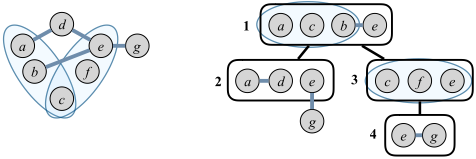
e g
a b d e f c g a b d e f c g Figure 1: An example of a hypergraph H = (V, E) (left) and one of its possible hypertree decompositions D = (T, χD, λD) (right). The vertex g is omitted at bag 2, which does not violate T4, as the node has no descendants. A case of a Special Condition violation can easily be constructed, if we replace the hyperedge {b, e} in the root's edge cover by {e, g}. T1-T3 would still hold, but as g occurs in a bag of a leaf, T4 gets violated. Furthermore, this conflict could not be resolved by adding g to bag 1, as that would violate T3, since g does not occur in bag 3.
- T4 If a vertex v is omitted at t, then it must not appear in the bag χD(t′ ) of any descendant node t′ of t.
In other words, T4 states that if t, t′ ∈ V (T) are nodes such that t′ is a descendant of t, then for each e ∈ λD(t) we have (e \ χD(t)) ∩ χD(t′ ) = ∅. The hypertree width htw(H) of H is the smallest width over all hypertree decompositions of H. See Fig. 1 for an example.
If the decomposition does not satisfy the Special Condition, then one speaks of a generalized hypertree decomposition, and one can define accordingly the generalized hypertree width ghtw(H) of H as the smallest width over all generalized hypertree decompositions of H. Clearly ghtw(H) ≤ htw(H). It is already NP-hard to decide whether a given hypergraph has generalized hypertree width ≤ 2 [Fischl et al., 2018], hence dropping the Special Condition increases the parameterized complexity of the recognition problem from XP to para-NP. The even more general parameter fractional hypertree width (with the same para-NP-hard recognition problem [Fischl et al., 2018]) arises when one considers fractional edge covers of the bags instead of edge covers [Grohe and Marx, 2014]. Recently powerful decomposers have been developed for these parameters beyond hypertree width [Fichte et al., 2018; Korhonen et al., 2019].
To avoid trivial cases, we consider only hypergraphs H = (V,E) where each v ∈ V is contained in at least one e ∈ E. Consequently, every considered hypergraph H has an edge cover, and htw(H) is always defined. If |V | = 1 then htw(H) = ghtw(H) = 1.
In the following, we also assume that each considered hypergraph is connected (i.e., its primal graph is connected). One can easily adapt our results to disconnected hypergraphs by operating component-wise.
3 Elimination Orderings for HTWidth
For this section, we consider a fixed, connected hypergraph H = (V, E). Consider a linear ordering v1 ≺ · · · ≺ vn of V . We think of the ordering as an elimination ordering in the usual sense: we eliminate one vertex after the other from the primal graph. Each time a vertex vi is eliminated, we make all its (remaining) neighbors adjacent (see, for example, [Bodlaender,


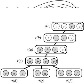
2005]), where newly added edges are referred to as fill-in edges. For our purposes and the forthcoming encoding, it is convenient to consider this elimination process on a directed version of the primal graph, where edges are oriented with respect to the linear ordering.
To that effect, let A ⊆ V ×V be the smallest set such that (i) if {u, v} ∈ E(P(H)) and u ≺ v then (u, v) ∈ A; and (ii) if (u, v) ∈ A, (u,w) ∈ A and v ≺ w then (v,w) ∈ A. Furthermore, for each v ∈ V (H), we define a set
Let A∗ denote the transitive closure over A, i.e., the smallest set containing A with the property that whenever (u, v) ∈ A∗ and (v, w) ∈ A∗ , then also (u, w) ∈ A∗ .
From the ordering one can construct a generalized hypertree decomposition D = (T, χD, λD), by taking for each v ∈ V (H) a tree node τ(v). We choose τ(r) for the ≺-largest vertex r as the root, and we set E(T) = { {τ(u), τ(w)} | w is the ≺-smallest vertex such that (u,w) ∈ A}. We call T the canonical tree for ≺. We further set χD(τ(u)) = χ≺(u) and let λD assign each node τ(u) a smallest edge cover of the set χD(τ(u)) with respect to H. Fig. 2 (bottom) shows an example of such a decomposition. Here, we can see an inherent problem of this translation that we need to address ("accumulating hyperedges"): The bag of the root cannot be covered without violating T4, as any vertex adjacent to c occurs in the bag of some descendant. In general this problem can occur anywhere in the decomposition, not only at the root. In the example we can resolve the problem by adding the white vertices. We observe that even when we ignore the redundant bags above τ(e), we do not get the same decomposition as in Fig. 1, since this decomposition tree is not the canonical tree of any ordering.
We will introduce a construction that circumvents this obstacle in general. To this aim, we need some further concepts and considerations.
For any two vertices u, w ∈ V (H), such that u ≺ w, we define their arc-path
and we say a vertex w ∈ V (H) is arc-reachable from u if (u,w) ∈ A∗ . In Fig. 2 (top), we can find arc-paths by simply following the arcs from left to right. This illustrates the motivation for arc-paths: whenever one vertex is arc-reachable from another, they have a descendency relationship in the corresponding decomposition.
We now introduce the aforementioned construction: we divide the forbidden vertices-vertices that would violate the Special Condition-at vertex w into two disjoint sets B(w) and B′ (w). We assume a mapping λ≺ that assigns an edge cover for χ≺ to each vertex:
The exceptional case discussed above is encapsulated in the definition of B′ (w): whenever every vertex on the arc-path between u and w has as its edge cover a superset of u's edge cover, we can omit u at w. If this property holds, we can repair any violation of the Special Condition, as we can add χ≺(u) to all the bags along the arc-path.
In Fig. 2 (bottom), B′ is represented by the white vertices. For the root, B consists of all vertices except c and the white vertices.
These definitions in hand, we can now give the LEOcharacterization of hypertree width.
Definition 1 (Hypertree Orderings). A hypertree ordering of H is a pair (≺, λ≺) where ≺ is a linear ordering of V and λ≺ is a mapping, assigning to each vertex v an edge cover for χ≺(v), such that the following properties hold:
We define the width of the hypertree ordering as maxv∈V |λ≺(v)|.
Condition O1 states that λ≺ assigns edge covers to the respective vertices. O2 defines the Special Condition, where the case distinction discussed above is implicit in the definition of B.
Theorem 2. The hypertree width of a hypergraph equals the minimum width over all its hypertree orderings.
We establish the theorem in an algorithmic way, by showing that we can transform in polynomial time a hypertree decomposition into a hypertree ordering of the same width, and conversely, that we can transform a hypertree ordering into a hypertree decomposition of the same width.
Let D = (T, χD, λD) be a hypertree decomposition of width W for a hypergraph H. We will translate D into an ordering O and show that O is a hypertree ordering of width W.
We first introduce the following terminology. A vertex v is forgotten at node t, if v ∈ χD(t), but v is not in the bag of t's parent. Every vertex in the bag of the root node, is forgotten at the root. We observe that each vertex v is forgotten at exactly one node t due to T3, hence we can write f(v) = t. We assume, w.l.o.g, that the following properties hold for D:
N1 For all t ∈ V (T), e ∈ λD(t): e ∩ χD(t) ̸= ∅.
N2 For all {t, t′ } ∈ E(T), if t′ is the parent of t then χD(t) ̸⊆ χD(t′ ).
We observe that N1 can be established by removing all violating hyperedges from the respective covers. N2 can be established by contracting edges between violating nodes and retaining the parent's cover and bag. Due to this property, at least one vertex is forgotten at every node.
Next, we define a preorder ⪯∗ on V (H) by setting v ⪯∗ w if and only if f(v) is in the subtree rooted at f(w) (this includes the case f(v) = f(w)). By letting ≺ be any total ordering that refines ⪯∗ and setting λ≺(v) := λD(f(v)), we define O = (≺, λ≺).
Proposition 3. O is a hypertree ordering of width W for the hypergraph H.
We now proceed and show the other direction. Given a hypertree ordering O = (≺, λ≺) of H, we define D = (T, χD, λD) by taking the canonical tree T as above by setting V (T) := { τ(v) | v ∈ V (H) }, E(T) := {{τ(u), τ(w)} | w is the ≺ -smallest vertex such that (u,w) ∈ A}, and by defining for all v ∈ V (H), λD(τ(v)) = λ≺(v) and
This definition implies that for every v ∈ V (H), f(v) = τ(v). Proposition 4. D = (T, χD, λD) is a hypertree decomposition of width W for H.
Propositions 3 and 4 establish Theorem 2.
4 SAT Encoding
In this section, we utilize the new LEO characterisation of hypertree width for an efficient SAT encoding. In the basic setup we follow closely the SAT encoding for treewidth as proposed by Samer and Veith [2009], variants of which served as the basis for several other encodings, for treewidth and other width measures [Bannach et al., 2017; Berg et al., 2017; Fichte et al., 2018; Lodha et al., 2017]. We note in passing, that the challenge of finding a characterisation of hypertree width that can be put on top of the Samer-Veith encoding of treewidth was our original motivation to pursue this work.
Again, we assume a given hypergraph H = (V, E) with n vertices v1, . . . , vn, and m hyperedges e1, . . . , em, and a bound W on the hypertree width. The task is to produce a propositional formula in Conjunctive Normal Form F(H,W), which is satisfiable if and only if htw(H) ≤ W. The construction will allow us to efficiently transform a satisfying assignment to F(H,W) into a hypertree ordering, and in turn into a hypertree decomposition of width ≤ W.
First, we review the basic setup following Samer and Veith's (2009) treewidth encoding. We express ≺ by using (n2 ) Boolean variables oi,j for 1 ≤ i < j ≤ n, where oi,j is true if and only if vi ≺ vj. We use the shorthand o∗i,j which stands for oi,j if i < j, and ¬oj,i otherwise. We establish transitivity by adding for all mutually distinct 1 ≤ i, j, k ≤ n the clause ¬o∗i,j ∨ ¬o∗j,k ∨ o∗i,k .
We define A using n(n - 1) Boolean variables ai,j, for distinct 1 ≤ i, j ≤ n, where ai,j is true if and only if (vi, vj) ∈ A. We add the clause ¬o∗i,j ∨ ¬aj,i for all distinct pairs 1 ≤ i, j ≤ n, to determine the direction of the arcs.
We initialize A with the edges from E(P (H)) by adding for all distinct pairs 1 ≤ i, j ≤ n, such that {vi, vj} ∈ E(P(H)), the clause ¬o∗i,j ∨ ai,j .
We finish the definition of A by encoding the fill-in edges: for all mutually distinct 1 ≤ i, j, k ≤ n we add the clause ¬o∗j,k ∨ ¬ai,j ∨ ¬ai,k ∨ aj,k.
We encode λ≺ and thereby O1 with nm weight variables wi,k, for 1 ≤ i ≤ n and 1 ≤ k ≤ m, where wi,k is true if and only if ek ∈ λ≺(vi). For the SMT encoding, instead of Boolean variables, we use integer valued variables. These integer variables can take the values 1 and 0, corresponding to true and false. For all distinct pairs 1 ≤ i, j ≤ n we add the clauses ¬ai,j ∨ ∨ek∈E,vj∈ek wi,k and ∨ek∈E,vi∈ek wi,k (for the SMT encoding, we replace the literal wi,k by wi,k ≥ 1).
We now encode the Special Condition, using property O2 of Definition 1. We define A∗ by n(n-1) Boolean variables bi,j , for distinct pairs 1 ≤ i, j ≤ n, where bi,j is true if and only if (vi, vj) ∈ A∗ . First, we add the arcs from A to A∗ . For all distinct pairs 1 ≤ i, j ≤ n we add the clause ¬ai,j ∨ bi,j . We obtain the transitive closure by adding for mutually distinct 1 ≤ i, j, k ≤ n the clause ¬aj,k ∨ ¬bi,j ∨ bi,k.
Next, we encode the exceptions B′ by adding n(n - 1) Boolean variables si,j , for distinct 1 ≤ i, j ≤ n, where si,j is true if and only if for every vertex vk on the arc-path between vi and vj it holds that λ≺(vi) ⊆ λ≺(vk). We first encode that every hyperedge in the edge cover of vi must also occur in the edge cover of vj , thereby ensuring λ≺(vi) ⊆ λ≺(vj). We add for all distinct pairs 1 ≤ i, j ≤ n and 1 ≤ k ≤ m the clause ¬si,j ∨ ¬wj,k ∨ wi,k.
We must ensure that this subset property holds along the whole arc-path. We express this by stating that the property only holds for vk, if it holds for all predecessors vj ∈ P(vi, vk) along the path. We add for mutually distinct 1 ≤ i, j, k ≤ n the clause ¬bi,j ∨ ¬bj,k ∨ ¬si,k ∨ si,j .
The Special Condition can be concisely stated with these two sets of variables. Whenever we have a vertex vj that is arc-reachable from vi, we prohibit the use of any hyperedge containing vi in the edge cover of vj. The only exception is the case, when the edge cover of every vertex on the arc-path is a superset of vi's edge cover. We add for distinct pairs 1 ≤ i, j ≤ n and ek ∈ {ek ∈ E(H) | vi ∈ ek }, the clause ¬bi,j ∨ sj,i ∨ ¬wj,k.
It remains to encode that each bag has an edge cover of size ≤ W. We implement this in two variants: (i) by expressing the cardinalities directly in SAT (as by Samer and Veith [2009] in the context of treewidth), and (ii) by using the more abstract handling of cardinalities by the algebraic theory solver within the SMT approach (as by Fichte et al. [2018] in the context of fractional hypertree width). In our SMT encoding, we can encode the necessary constraints for i ≤ n directly as ∑ek∈E wi,k ≤ W. For our SAT encoding, we use totalizer cardinality constraints [Bailleux and Boufkhad, 2003]. These performed best among all cardinality constraints provided by PySAT [Ignatiev et al., 2018] and are inherently compatible with incremental SAT solving [Martins et al., 2014].
We also use our encoding in conjunction with MaxSAT. Given variables ci,k, 1 ≤ i ≤ n, 1 ≤ k ≤ W, defined by the cardinality constraints, where ci,k is true if |λ≺(vi)| ≥ k. We add variables mk for 1 ≤ k ≤ W, where mk is true if the hypertree width is less than k. We ensure the semantics of m by adding for 1 ≤ i ≤ n, 1 ≤ k ≤ W the clauses ¬mk ∨¬ci,k. Finally, we let the solver minimize the width by adding for 1 ≤ k ≤ W the weighted clauses mk.
The correctness of the encoding follows by construction and Theorem 2. Obviously, the SAT/SMT formula F(H,W) can be constructed in polynomial time, given H and W, hence we arrive at the following result.
Theorem 5. Given a hypergraph H with n vertices and m hyperedges and an integer W, we can construct in time polynomial in n +m+W a SAT/SMT formula F(H,W) which is satisfiable if and only if htw(H) ≤ W.
Asymptotically, the number of clauses is in O(n3 ), which is similar to other encodings for structural decompositions [Fichte et al., 2018; Samer and Veith, 2009; Schidler and Szeider, 2020]. However, the actual constants have a significant influence on performance and scalability of the encoding, and we can observe that our encoding requires less than half the number of clauses compared with the encoding by Schidler and Szeider [2020].
Improvements. The encoding of the Special Condition follows the definition of O2 to show its correctness by construction. We can encode it more succinctly, by encoding O2 in a less direct way.
This improvement uses two ideas. The first idea is, we do not encode the forbidden, but the permitted vertices, i.e. V (H) \ B(v). This makes it possible to use only one set of variables that combines bi,j and si,j. The other idea is to restrict the vertices we consider for B′ .
We use n(n- 1) variables pi,j , for distinct pairs 1 ≤ i, j ≤ n, where pi,j is true if and only if vi is permitted in the edge cover of vj. We restrict the use of hyperedges in the edge covers as before, by adding for all distinct pairs 1 ≤ i, j ≤ n and ek ∈ { ek ∈ E(H) | vi ∈ ek } the clause pi,j ∨ ¬wj,k.
We also enforce, that the allowed property holds along arcpaths. This is similar to the encoding of A∗ , but combined with the subset-path property. We add for mutually distinct 1 ≤ i, j, k ≤ n the clauses ¬aj,k ∨ pi,j ∨ ¬pi,k.
It remains to encode the conditions that define when a vertex is forbidden. Due to the following result, we can restrict the scope of subset paths.
Proposition 6. Let u ∈ V (H) and v be the ≺-largest vertex, such that (u, v) ∈ A: For every vertex w such that v ≺ w, we can remove any hyperedge containing u from λ≺(w).
Using this result, we can discard all vertices that are not direct successors of vi. We add for all mutually distinct 1 ≤ i, j, k ≤ n the clause ¬ai,j ∨ ¬aj,k ∨ ¬o∗i,k ∨ ai,k ∨ ¬pi,k.
It remains to check the subset property. As before, we add
for distinct pairs 1 ≤ i, j ≤ n and 1 ≤ k ≤ m the clause
¬ai,j ∨ ¬pi,j ∨ ¬wi,k ∨ wj,k.
5 Experiments
Results 3 and code 4 of the experiments are available online.
Experimental Setup. We implemented the improved encoding presented in Section 4 using Pysat 1.6.0 5 and refer to it as HtdLEO. We compared our encoding to the encoding HtdSMT by Schidler and Szeider [2020] 6 . Both versions were run using Python 3.8.0. We compared the encoding-based approaches with the state-of-the-art decomposer det-k-decomp 7 by Gottlob and Samer [2009], which implements an XP-algorithm based on dynamic programming over separators.
We used the following solvers. Optimathsat 1.7.2 8 was used for the SMT encodings, as it performed better than z3 4.8.9. We used Glucose 3 for SAT instances, as it performed best among the solvers implemented by PySAT. MaxSAT instances were solved by UwrMaxSAT 9 , the winner of the MaxSAT Evaluation 2020 10 . For the SAT encoding, we start at an initial heuristically computed width. This width is then decremented until the formula is unsatisfiable. We used servers with two Intel Xeon E5540 CPUs, each running at 2.53 GHz per core. The servers used Ubuntu 18.04. Each run was limited to thirty minutes and 8 GB RAM. In the results each non-solved instance is counted as thirty minutes towards the total runtime.
Benchmark Instances. We tested against the full set of Hyperbench 11 instances. Hyperbench consists of instances gathered from various database queries and constraint satisfaction problem instances [Fischl et al., 2019; Bonifati et al., 2017; Bonifati et al., 2019; Pottinger and Halevy, 2001; Benedikt et al., 2017], for which hypertree width is of practical relevance. The instances of the PACE 2019 competition form a subset of the Hyperbench instances. We removed all disconnected and single-vertex instances and ran each configuration against the remaining 3008 instances. 2019 of these instances were solved by any solver and 840 were solved by all solvers. We present the results for the 2019 solved instances.
Experimental Results. In Table 1 we see a summary of how many instances the different configurations and solvers were able to solve. We were interested to see, whether the different configurations solved mostly the same, or different instances. This is shown in the Unique column. We also looked at the performance of the configurations based on the hypertree width of the instances. Table 2 shows the number of solved instances for each configuration grouped by hypertree width.
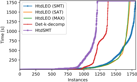
We can see that the SMT encoding performs better than the SAT encoding. In Table 2 we see that this is mainly because the SMT encoding is more stable for instances with larger hypertree width. The SAT encoding performs considerably better for smaller widths with an almost absolute drop at width 6.
3 doi.org/10.5281/zenodo.4742069
4 github.com/ASchidler/htdsmt, doi.org/10.5281/zenodo.4742100
5 pysathq.github.io
6 github.com/ASchidler/frasmt pace/ (Commit f789760)
7 github.com/daajoe/detkdecomp (Commit 277d593)
8 optimathsat.disi.unitn.it
9 github.com/marekpiotrow/UWrMaxSat (Commit: 0f152ee)
10 maxsat-evaluations.github.io
11 hyperbench.dbai.tuwien.ac.at/
| Solver | # Solved | Time [s] | Unique |
|---|---|---|---|
| HtdLEO (SMT) | 1810 (90%) | 1217.3 | 128 |
| HtdLEO (SAT) | 1723 (85%) | 1244.3 | 26 |
| HtdLEO (MAX) | 1706 (84%) | 1251.5 | 5 |
| Det-k-decomp | 1378 (68%) | 1545.3 | 21 |
| HtdSMT | 1211 (60%) | 1679.1 | 1 |
| Solver | 1 | 2 | 3 | 4 | 5 | 6 | >6 |
|---|---|---|---|---|---|---|---|
| 461 | 223 | 306 | 378 | 370 | 273 | 8 | |
| HtdLEO (SMT) | 449 | 209 | 262 | 301 | 333 | 255 | 1 |
| HtdLEO (SAT) | 461 | 216 | 305 | 373 | 341 | 27 | 0 |
| HtdLEO (MAX) | 457 | 215 | 305 | 371 | 333 | 25 | 0 |
| Det-k-decomp | 461 | 223 | 306 | 319 | 34 | 28 | 7 |
| HtdSMT | 342 | 161 | 165 | 179 | 245 | 119 | 0 |
The behavior is more clearly visible in Fig. 3: the SAT encoding solves most instances either quickly or not, while the SMT encoding's runtime increases more slowly. This may be either due to a generally different internal processing in the SMT solver compared to the SAT solver or the arithmetic constraints causing a different solving process. The MaxSAT encoding performs very similar to the SAT encoding, as is visible in Fig. 3. Nonetheless, Table 2 suggests some differences. Indeed, there are 23 instances solved using MaxSAT that could not be solved by the SAT encoding, which was able to solve 40 instances that the MaxSAT encoding was unable to solve. When counting MaxSAT and SAT as a single approach, this approach solves 90 instances that no other solver solved. When comparing only SMT and SAT, SMT solved 267 unique instances and SAT 180. This indicates that a portfolio approach combining SAT and SMT encodings may be a good option to solve more instances in total.
The comparison to other decomposers shows that our new approach outperforms both the old encoding HtdSMT [Schidler and Szeider, 2020] and det-k-decomp [Gottlob and Samer, 2009] by a large margin when we compare the total number of solved instances. While HtdLEO is strictly better than HtdSMT, as the latter could solve only one instance uniquely, we have a different picture for det-k-decomp. Some instances were uniquely solved by det-k-decomp. We can see in Tables 1 and 2 that the behavior of det-k-decomp is similar to the SAT encoding, in terms of the instances they solved and in terms of the correlation between hypertree width and number of solved instances. The main difference is, that for det-k-decomp the significant drop already occurs at hypertree width 5.
6 Concluding Remarks
We presented the first characterisation of hypertree width that is purely based on linear elimination orderings (LEO), in contrast to previous characterisations which require auxiliary structures. This characterization provides new combinatorial insights into hypertree decompositions. We utilized the characterisation for a new SAT/SMT encoding and tested it on an extensive set of benchmark instances. Indeed, the new encoding clearly outperforms the existing encoding, as well as the state-of-the-art combinatorial algorithm for hypertree decompositions. We expect that the new LEO-based characterisation of hypertree width will also be of interest outside SAT encodings, for instance, for Branch & Bound algorithms.
As mentioned in the introduction, the recognition of hypergraphs of hypertree width W is XP-tractable when parameterized by W, but the corresponding problem for generalized hypertree width is para-NP-hard. This complexity-theoretic perspective suggests that the former problem is easier than the latter. When considering SAT encodings, Schidler and Szeider [2020] observed that the opposite seems to prevail. Whereas generalized hypertree width was captured by a relatively simple and compact encoding, the Special Condition required a complicated characterisation, resulting in a significantly less efficient encoding. With our new LEO characterisation of hypertree width, we were able to, at least partially, resolve this apparent discrepancy between theory and practice. When we compare HtdLEO with a plain generalized hypertree width encoding, we see a similar number of solved instances 12 .
We hope that in the future one can build upon our LEO characterisation and encoding, and develop further improvements, including preprocessing and inprocessing techniques, so that optimal hypertree decompositions can be efficiently found for even larger instances.
Acknowledgements
The authors acknowledge the support from the FWF (P32441, W1255) and the WWTF (ICT19-065).
12 A SAT encoding for ghtw solves 1664 instances, compared to 1723 solved by HtdLEO (SAT); an SMT encoding solves 1795 instances, compared to 1810 solved by HtdLEO (SMT).
@inproceedings{ijcai2021p196,
  title     = {Computing Optimal Hypertree Decompositions with SAT},
  author    = {Schidler, Andre and Szeider, Stefan},
  booktitle = {Proceedings of the Thirtieth International Joint Conference on
               Artificial Intelligence, {IJCAI-21}},
  publisher = {International Joint Conferences on Artificial Intelligence Organization},
  editor    = {Zhi-Hua Zhou},
  pages     = {1418--1424},
  year      = {2021},
  month     = {8},
  note      = {Main Track},
  doi       = {10.24963/ijcai.2021/196},
  url       = {https://doi.org/10.24963/ijcai.2021/196},
}
TY - CPAPER TI - Computing Optimal Hypertree Decompositions with SAT AU - Schidler, Andre AU - Szeider, Stefan T2 - Proceedings of the Thirtieth International Joint Conference on Artificial Intelligence, IJCAI-21 PB - International Joint Conferences on Artificial Intelligence Organization PY - 2021 SP - 1418 EP - 1424 DO - 10.24963/ijcai.2021/196 UR - https://doi.org/10.24963/ijcai.2021/196 ER -Copied
Machine-readable versions of this paper, for tools and AI agents:





