
Approximating the Shapley Value Using Stratified Empirical Bernstein Sampling
Proceedings of the Thirtieth International Joint Conference on Artificial Intelligence. Main Track. Pages 73-81.
https://doi.org/10.24963/ijcai.2021/11
Keywords
- Agent-based and Multi-agent Systems: Cooperative Games
- Uncertainty in AI: Uncertainty Representations
Abstract
The Shapley value is a well recognised method for dividing the value of joint effort in cooperative games. However, computing the Shapley value is known to be computationally hard, so stratified sample-based estimation is sometimes used. For this task, we provide two contributions to the state of the art. First, we derive a novel concentration inequality that is tailored to stratified Shapley value estimation using sample variance information. Second, by sequentially choosing samples to minimize our inequality, we develop a new and more efficient method of sampling to estimate the Shapley value. We evaluate our sampling method on a suite of test cooperative games, and our results demonstrate that it outperforms or is competitive with existing stratified sample-based estimation approaches to computing the Shapley value.
- [Audibert et al., 2007] Jean-Yves Audibert, Rémi Munos, and Csaba Szepesvári. Tuning bandit algorithms in stochastic environments. In Marcus Hutter, Rocco A. Servedio, and Eiji Takimoto, editors, Proceedings of the 18th International Conference on Algorithmic Learning Theory (ALT'07), pages 150-165, Berlin, Heidelberg, 2007. Springer Berlin Heidelberg.
- [Audibert et al., 2009] Jean-Yves Audibert, Rémi Munos, and Csaba Szepesvári. Exploration-exploitation tradeoff using variance estimates in multi-armed bandits. Theoret- ical Computer Science, 410(19):1876-1902, 2009.
- [Aziz et al., 2016] Haris Aziz, Casey Cahan, Charles Gret- ton, Philip Kilby, Nicholas Mattei, and Toby Walsh. A study of proxies for Shapley allocations of transport costs. Journal of Artificial Intelligence Research, 56:573-611, 2016.
- [Bachrach et al., 2009] Yoram Bachrach, Evangelos Markakis, Ezra Resnick, Ariel D. Procaccia, Jeffrey S. Rosenschein, and Amin Saberi. Approximating power indices: theoretical and empirical analysis. Autonomous Agents and Multi-Agent Systems (AAMAS), 20:105-122, 2009.
- [Bardenet and Maillard, 2015] Rémi Bardenet and Odalric- Ambrym Maillard. Concentration inequalities for sam- pling without replacement. Bernoulli, 21(3):1361-1385, 08 2015.
- [Bennett, 1962] George Bennett. Probability inequalities for the sum of independent random variables. Journal of the American Statistical Association, 57(297):33-45, 1962.
- [Boucheron et al., 2003] Stephane Boucheron, Gábor Lu- gosi, and Pascal Massart. Concentration inequalities us- ing the entropy method. The Annals of Probability, 31(3):1583-1614, 2003.
- [Carpentier et al., 2011] Alexandra Carpentier, Alessandro Lazaric, Mohammad Ghavamzadeh, Rémi Munos, and Peter Auer. Upper-confidence-bound algorithms for ac- tive learning in multi-armed bandits. In Proceedings of the 22nd International Conference on Algorithmic Learn- ing Theory (ALT'11), pages 189-203, Berlin, Heidelberg, 2011. Springer-Verlag.
- [Castro et al., 2009] Javier Castro, Daniel Gómez, and Juan Tejada. Polynomial calculation of the Shapley value based on sampling. Computers & OR, 36(5):1726-1730, 2009.
- [Castro et al., 2017] Javier Castro, Daniel Gómez, Elisenda Molina, and Juan Tejada. Improving polynomial estima- tion of the Shapley value by stratified random sampling with optimum allocation. Computers & Operations Re- search, 82:180 -188, 2017.
- [Chapman et al., 2017] Archie C. Chapman, Sleiman Mhanna, and Gregor Verbič. Cooperative game theory for non-linear pricing of load-side distribution network support. In Proceedings of the 10th Bulk Power Systems Dynamics and Control Symposium (IREP'17), 2017.
- [Efron and Stein, 1981] Bradley Efron and Charles Stein. The jackknife estimate of variance. Annals of Statistics, 9(3):586-596, 05 1981.
- [Hoeffding, 1963] Wassily Hoeffding. Probability inequal- ities for sums of bounded random variables. Journal of the American Statistical Association, 58(301):13-30, Mar 1963.
- [Lundberg and Lee, 2017] Scott M Lundberg and Su-In Lee. A unified approach to interpreting model predictions. In Advances in neural information processing systems, pages 4765-4774, 2017.
- [Maleki et al., 2013] Sasan Maleki, Long Tran-Thanh, Greg Hines, Talal Rahwan, and Alex Rogers. Bounding the Es- timation Error of Sampling-based Shapley Value Approxi- mation. arXiv e-prints, page arXiv:1306.4265, June 2013.
- [Maurer and Pontil, 2009] Andreas Maurer and Massimil- iano Pontil. Empirical Bernstein bounds and sample vari- ance penalization. In Proceedings of the 22nd Annual Con- ference on Learning Theory (COLT 2009), June 2009.
- [Michalak et al., 2013] Tomasz P. Michalak, Karthik V. Aa- dithya, Piotr L. Szczepanski, Balaraman Ravindran, and Nicholas R. Jennings. Efficient computation of the Shap- ley value for game-theoretic network centrality. Journal of Artificial Intelligence Research, 46(1):607-650, January 2013.
- [Mnih et al., 2008] Volodymyr Mnih, Csaba Szepesvári, and Jean-Yves Audibert. Empirical Bernstein stopping. In Proceedings of the 25th International Conference on Ma- chine Learning (ICML), ICML '08, pages 672-679, New York, NY, USA, 2008. ACM.
- [Neyman, 1938] J. Neyman. Contribution to the theory of sampling human populations. Journal of the American Statistical Association, 33(201):101-116, 1938.
- [O'Brien et al., 2015] Geaorid O'Brien, Abbas El Gamal, and Ram Rajagopal. Shapley value estimation for compen- sation of participants in demand response programs. IEEE Transactions on Smart Grid, 6(6):2837-2844, 2015.
- [Serfling, 1974] Robert J. Serfling. Probability inequalities for the sum in sampling without replacement. The Annals of Statistics, 2(1):39-48, 01 1974.
- [Soufiani et al., 2014] Hossein Azari Soufiani, Denis X Charles, David M Chickering, and David C Parkes. Ap- proximating the Shapley value via multi-issue decomposi- tion. In Proc. Autonomous Agents and Multi-Agent Sys- tems '14. ACM, 2014.
- [Thomas et al., 2015] Philip S. Thomas, Georgios Theocharous, and Mohammad Ghavamzadeh. High- confidence off-policy evaluation. In Proceedings of the 29th AAAI Conference on Artificial Intelligence, January 25-30, 2015, Austin, Texas, USA., pages 3000-3006, 2015.
References were extracted automatically from the PDF and may contain errors.
Full text extracted automatically from the PDF; figures, tables and equations may differ. The PDF is the version of record.
1 Introduction
The Shapley value is a cornerstone measure in cooperative game theory. It is an axiomatic approach to allocating a divisible reward or cost between participants where there is a clearly defined notion of how much surplus or profit a group or "coalition" of participants could achieve by themselves. It has many applications, including analyzing the power of voting blocks in weighted voting games [Bachrach et al., 2009], in cost and surplus division problems [Soufiani et al., 2014; O'Brien et al., 2015; Aziz et al., 2016; Chapman et al., 2017], as a measure of network centrality [Michalak et al., 2013]; and as a method of explaining the predictions of machine learning models [Lundberg and Lee, 2017]. Specifically, under the Shapley value, each player is allocated their average marginal contribution across every possible sequence of player join orderings. Although the Shapley value is conceptually simple, its use is hampered by the fact that its exact computation requires exponentially many evaluations of the marginal contributions of the players in the coalition.
Given this difficulty, one can exploit the fact that the Shapley value is an average by using estimation techniques to approximate it. In particular, the coalitions evaluated in the Shapley value computation can be naturally stratified by coalition size, allowing it to be reformulated as an average over strata averages. It is then possible to separately and efficiently estimate these strata averages via sample allocation techniques. Such techniques in literature include simple random sampling [Castro et al., 2009], simple stratified random sampling, and a Neyman-type allocation [Castro et al., 2017], and allocating stratified samples to minimize a Hoeffding type inequality [Maleki et al., 2013].
In this paper, we improve on these approaches by developing a method for stratified sampling to maximally reduce an expression of the uncertainty in the Shapley value estimate. To do this, we develop a general expression associated with that uncertainty, which takes the form of a concentration inequality; specifically, a stratified empirical Bernstein bound (SEBB). This inequality considers factors such as: the sizes of all the strata and the proportion of each that are sampled; the sample variances of the samples from each of the strata; the differences in the range of data of each strata; any additional importance weightings on the strata, and; whether any (or all) of the strata are sampled with or without replacement.
Using our SEBB, we propose an online method for sequentially sampling in order to maximally reduce the bound at each iteration, called the stratified empirical Bernstein method (SEBM). We numerically demonstrate the value of the SEBM by using it to compute the Shapley value in a suite of benchmark cooperative games. Our comparisons to existing sample-based approaches to computing the Shapley value show that our method is almost uniformly superior.
Next, Section 2 frames some context of the paper. Section 3 provides several component lemmas. From this Section 4 provides the derivation of our concentration inequality. In Section 5, we evaluate the performance of our bound in approximating the Shapley value. Section 6 discusses a multidimensional extension to the concentration inequality, and Section 7 concludes.
2 Background
Stratified sampling is a well known sampling technique, which estimates the mean of a population by partitioning it into mutually exclusive subgroups, or strata. It proceeds by applying a sampling estimator to each stratum, before weighting and combining these estimates to form an estimate of the population mean. If strata and their sizes are naturally given or determined, there exists a further question of how to allocate the sampling between the strata.
One way of deriving a sampling method is to use a concentration inequality as a confidence bound on the error of the population mean, and then selecting additional samples to minimise it. For instance, minimising Chebyshev's inequality on the variance of the estimation of the population mean results in the well-known Neyman allocation [1938], which has been inspiration as a method of estimating the Shapley value [Castro et al., 2017]. Hoeffding's inequality is another commonly used concentration inequality whose minimisation has also been adapted in the context of Shaplay value sampling [Maleki et al., 2013].
Recently, there has been interest in concentration inequalities called empirical Bernstein bounds (EBBs) [Maurer and Pontil, 2009], which are probabilistic bounds for the sample mean and sample variance. EBBs have been subject to rapid development [Audibert et al., 2009; Audibert et al., 2007; Bardenet and Maillard, 2015] and have replaced Hoeffding's inequality in a number of computational applications [Mnih et al., 2008; Thomas et al., 2015; Carpentier et al., 2011].
Sampling without replacement offers the opportunity to further tighten the concentration bounds over the samplingwith-replacement case. The refinement was first demonstrated with a martingale argument by Serfling [1974] which was recently improved to created an EBB suitable for sampling without replacement by Bardenet and Maillard [2015].
Our observation, is that the components of these analyses can be used to create a variance-sensitive concentration inequality tailored for stratified random sampling, which then can be minimised in the context of Shapley value estimation.
3 Preliminaries
We now state lemmas which we use to derive our stratified empirical Bernstein bound (SEBB); the proofs of lemmas and theorems are as supplemental documentation (section A). The first lemma is an often-used and rather weak result used to fuse simple statements of probability:
Lemma 3.1 (Probability Union). For any random variables:
The next lemma is a result of algebra that relates the sample squares about the mean to the sample variance.
Lemma 3.2 (Variance Relation). For random variable X with mean µ, and n samples {xk}k=1,...,n. The sample mean ˆµ = 1n ∑k xk, sample variance, ˆσ2 = 1n ∑k (xk - ˆµ)2 , centered average sample squares ˆσ2 0 = 1n ∑k (xk - µ)2 , obey:
We use this result to create bounds for the sample variance from bounds on the sample squares. We also use the next lemma, which extends directly from Markov's inequality:
Lemma 3.3 (Chernoff Bound). For a random variable X, and for any s > 0 and t:
Many well-known inequalities follow from upper bounds for E [exp(sX)], also known as the moment generating function.
3.1 Bounds on the Moment Generating Function
The next three lemmas give three upper bounds for moment generating functions. The first is the famous Hoeffding's lemma [1963] which is essentially constructed by fitting a line over the exponential function of the moment generating function:
Lemma 3.4 (Hoeffding's Lemma). For random variable X bounded a ≤ X ≤ b with D = b - a, for any s > 0:
The next is a similar bound on the moment generating function that involves information about the variance.
Lemma 3.5. For random variable X bounded a ≤ X ≤ b with D = b - a and variance σ2 , for any s > 0:
The proof of this lemma is provided in supplementary material (section A), and essentially involves fitting a parabola (instead of a line) over the exponent in the moment generating function. This lemma is a simplified half-way result used in a derivation of Bennett's inequality as presented by Hoeffding [1963], and derived by Bennett [1962].
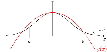
The next lemma stems from the creation of an upper bound on the random variable -X2 instead of X. In this context the moment generating function becomes the expectation value of a Gaussian function which can be bound above by a parabola, yielding:
Lemma 3.6. For random variable X bounded a ≤ X ≤ b, with D = b - a and variance σ2 ,and for any q > 0:
The three inequalities above (Lemmas 3.4, 3.5 and 3.6) are used in the derivation of our stratified sampling concentration inequality in Section 4.
3.2 Moment Generating Function of Means
In the previous subsection we considered bounds on the moment generating function of random variables, but we must also relate these to bounds on the moment generating function of sample means from that of the random variables. The first is the most straightforward way to do this in the case of sampling with replacement, and directly assumes the independence of the samples:
Lemma 3.7 (Replacement Bound). For random variable X bounded a ≤ X ≤ b with a mean of zero, with D = b - a and variance σ2 . Let χm = 1m ∑mi=1 Xi be the average of m independently drawn (with replacement) samples. If there exists an α, β ≥ 0 such that for any s > 0 that
then:
However, for the context of sampling without replacement, there is an alternative result which can be substituted and may be (or may not be) tighter. In this context substituting one for the other can be done judiciously on a case-by-case basis to create the tightest possible bound. All the numerical results in this paper have been produced with this judicious choice conducted. This result directly extends a reverse martingale argument fromBardenet and Maillard [2015]:
Lemma 3.8 (Martingale Bound). For finite data set x1, x2, . . . xn that is bounded a ≤ xi ≤ b, and has a mean of zero and variance σ2 = 1n ∑ni=1 x2i , denote X1,X2, . . . ,Xn the random variables corresponding to the data sequentially drawn randomly without replacement, and χm the average of the first m of them.
where
and
Under the assumption that for any random variable Z with a mean of zero such that a ≤ Z ≤ b and D = b - a, with variance σ2Z that there exists an α, β ≥ 0 such that for any s > 0 that E[exp(sZ)] ≤ exp((αD2 + βσ2Z )s2 ).
Proofs of both of these lemmas are found in supplementary material (section A).
4 The Stratified Finite Empirical Bernstein Bound and Sampling Method
We derive a novel probability bound for the error of the stratified sampling estimate, we begin by precisely defining the context of our derivations, to which our bound applies.
Definition 4.1 (Problem context). Let a population consist of n number of strata of finite data points, where ni is the number of data points in the ith stratum. All values in a stratum are bound within a finite support of width Di. Denote the mean and variance of the ith stratum µi and σ2 i , respectively. Denote random variables for values sequentially drawn (with or without) replacement as Xi,1,Xi,2, . . . ,Xi,ni . Then, for the first mi of these samples:
- χi,mi = 1 mi ∑mi j=1 Xi,j is their average;
- their biased sample variance is ˆσ2 i = 1 mi ∑mi j (Xi,j - χi,mi )2 , and;
- their unbiased sample variance is ˆˆσ2 i =miˆσ2 i /(mi -1).
We are interested in the average of the means of the strata as weighted by constant positive factors {τi}i∈{1...n}. In the derivation we use arbitrary positive variables {θi}i∈{1...n}.
Given this context, the following two sections contain the derivation of the stratified empirical Bernstein bound (SEBB) and the sequential sampling method (SEBM), respectively.
4.1 Bound Derivation
The bound is now developed in four theorems, which build on each other in sequence:
- Theorem 4.2 bounds the error in the stratified population mean estimate ∑ni=1 τiχi,mi in the context of variance information.
- Theorem 4.3 bounds the variance information in the context of sample variance information and the squared stratum mean errors.
- Theorem 4.4 bounds the squared stratummean errors.
- Theorem 4.5 combines the three previous theorems together using union bounds (to eliminate the dependence on variance information and squared stratum mean errors), to create a concentration inequality for the error in the stratified population mean estimate given the sample variance information.
We begin with an expression for a probability bound on the absolute error of the weighted stratified sample means about the weighted strata means, and is developed from lemma 3.5:
Theorem 4.2. Assuming the context given in Definition 4.1, and let Ωni mi and Ψni mi be given as in Lemma 3.7, then:
In most cases, the weights τi can be considered as the probability weights τi = ni/(∑nj=1 nj), and in this context this probability bound can be used as-is for a measure of uncertainty in stratified random sampling if the true variances (or alternatively, upper bounds on the true variances) of the strata are known. However, in other contexts, the weighted sum of variances must be estimated from the data collected, and to include this factor we develop and incorporate a probability bound for the estimate of the sum of variances (as weighted by arbitrary θi), as follows from use of Lemma 3.6.
Theorem 4.3. Assuming the context given in Definition 4.1. Then with Ψni mi per Lemma 3.7:
This inequality gives the probability bound between the weighted variances of the strata, the weighted (biased) sample variances and the weighted square error of the sample means. Although the weighted square error of the sample means may go to zero quickly as additional samples are taken, we nonetheless develop another probability bound to incorporate specific consideration of it, from lemma 3.4.
Theorem 4.4. Assuming the context given in Definition 4.1. Then with Ωni mi as in Lemma 3.7:
This theorem bounds the weighted square error of the sample means. In the next, and final, step we combine the inequalities of Equations (1), (2) and (3) together, to complete our derivation of the SEBB.
Theorem 4.5 (Stratified Empirical Bernstein Bound (SEBB)). Assuming the context given in Definition 4.1. Then with Ωni mi , Ψni mi per Lemma 3.7:
This completes the derivation. In Equation (4) of Theorem 4.5, we have a concentration inequality for the sum of weighted strata sample mean errors relative to the sample variances. In this context, the weights τi are flexible but would naturally be probability weights proportional to strata size, τi = ni/(∑nj=1 nj), in which case the inequality provides a concentration of measure in stratified random sampling. Based on this bound, we proceed to propose an online process of sequentially choosing samples from the strata in order to minimize it.
The derivation of our inequality extends from consideration of Chernoff bounds and probability unions in a similar vein to other EBB derivations [Maurer and Pontil, 2009; Bardenet and Maillard, 2015]. However, the various bounds on the moment generating functions that we developed in Section 3 use some loosening approximations in their derivations, and hence stronger and/or more representative bounds could be developed at the cost of greater mathematical complexity. Alternatively, integrating other kinds of inequalities such as entropic [Boucheron et al., 2003] or Efron-Stein [Efron and Stein, 1981] could result in different and potentially tighter bounds. Nonetheless, when we use this bound in a sequential sampling algorithm, as described next, we see clear-cut estimation efficiency improvements in the Shapley value estimation task, as demonstrated in Section 5.
4.2 Sequential Sampling using the Stratified Empirical Bernstein Method
We introduce a method of sampling, the stratified empirical Bernstein method (SEBM) which sequentially minimizes the bound in Theorem 4.5 (SEBB). Pseudocode for the calculation of the bound and the process of sampling to minimize it, is given in Algorithm 1.
Algorithm 1 Stratified Empirical Bernstein Method (SEBM) with replacement
Require: probability p, strata number N, stratum sizes ni, initial sample numbers mi, initial stratum sample variances ˆˆσ2 i , weights τi, widths Di, sample budget B
1: while ∑i mi < B do 2: beststrata ←-1 3: lowestbound ← ∞ 4: for k = 0 to N do 5: mk ←mk +1 6: a ← [0, 0], b ← [0, 0], c ← [0, 0], d ← [0, 0] 7: for i = 0 to N do 8: Ωmin ← min( ¯Ωni mi , Ωni mi ) 9: Ψmin ← min( ¯Ψni mi , Ψni mi ) 10: a0 ← a0 + log(6N/p)D2 i ¯Ψni mi Ωminτ 2 11: a1 ← a1 + log(6N/p)D2 i Ψni mi Ωminτ 2 12: b0 ← max(b0, log(3/p)D2 i ¯Ψni mi Ψminτ 2 ) 13: b1 ← max(b1, log(3/p)D2 i Ψni mi Ψminτ 2 ) 14: c0 ← c0 + 2 ¯Ψni mi ((mi - 1)ˆˆσ2 i /mi)τ 2 15: c1 ← c1 + 2Ψni mi ((mi - 1)ˆˆσ2 i /mi)τ 2 16: d0 ← d0 + 4 17 D2 i ¯Ωni mi τ 2 17: d1 ← d1 + 4 17 D2 i Ωni mi τ 2 18: end for 19: w ← √minj(dj + (√cj +aj + bj + √bj)2 ) 20: if w < lowestbound then 21: beststrata ← k 22: lowestbound ← w 23: end if 24: mk ←mk -1 25: end for 26: take an extra sample from strata: beststrata 27: mbeststrata ←mbeststrata +1 28: recalculate ˆˆσ2 beststrata 29: end whileSpecifically, Algorithm 1 is a repetitive process involving a scan through the possible strata and then the selection of one stratum to sample from to minimize the SEBB under mild assumptions. The process of scanning involves calculating the confidence bound width (SEBB) that would result if an additional sample were to be taken from that stratum without changing its sample variance (line numbers 5-17 in Algorithm 1). The stratum that yields the smallest confidence bound width in the context of an additional sample is then selected (line 18-21) and sampled (line 24), the sample variance of that stratum is updated (line 26); this process repeats until the maximum sample budget is reached (per the outer loop, line 1). In this way the process attempts to iteratively minimize the SEBB in expectation with each additional sample taken; and hence lead to potentially greater accuracy in stratified sampling as a result.
We note that computing the SEBB requires the sample variances of all the strata having been calculated. Accordingly, Algorithm 1 must be initialized with at least two samples from each stratum so that sample variance can be calculated.
Algorithm 1 describes a process specific to sampling without replacement and involves the calculation of the SEBB with the tightest possible uses of Lemmas 3.8 and 3.7. In particular, for any stratum i that is sampled without replacement, any specific bound with an associated Ωni mi and Ψni mi may be substituted for ¯Ωni mi and ¯Ψni mi to potentially tighten the bound, and this corresponds to choice of Lemma 3.8 or Lemma 3.7 in the bound's derivation. Since the SEBB is a composition of such bounds with such choices throughout, there is a structure of valid pairs of substitutions Ω,Ψ for ¯Ω, ¯Ψ in the optimal calculation of the SEBB, which is shown in the steps 8-15 of Algorithm 1, using partial terms {a, b, c, d}. The equivalent algorithm for sampling with replacement simply is the same algorithm altered by replacing all use of ¯Ω, ¯Ψ with Ω, Ψ.
5 Numerical Evaluation: Shapley Value Approximation
We assess the benefits of using our sampling method by comparing its performance to other approaches in a set of example cooperative games.
For each game, we compute the exact Shapley value, and then the average absolute errors in the approximated Shapley value for a given budget of marginal-contribution samples across multiple computational runs. The results are shown in Table 1, where eSEBM is the error associated with our method, SEBM, which is compared to the average absolute error in the Shapley value by sampling with:
- A Hoeffding-bound method [Maleki et al., 2013], denoted eMa ,
- Simple random sampling of the without stratification, the described 'ApproShapley' method [Castro et al., 2009], denoted eapp
- The stratified simple sampling method 'StApproShapley' [Castro et al., 2017], denoted esim
- Castro's Neyman-type sampling method 'StApproShapley-opt' [Castro et al., 2017], denoted eCa
Next, we describe the example cooperative games, and then discuss our results.
5.1 Example Cooperative Games
In general, a cooperative game, 〈N, v〉 ∈ GN, comprises a set of n players, N = {1, 2, . . . , n}, and a characteristic function, v : S ⊂ N → R, which is a function specifying the reward which can be achieved if a subset of the players S ⊂ N cooperate, where v(∅) = 0. In this context the Shapley value ϕ is a unique mapping from cooperative games to the player rewards GN → Rn which satisfies many attractive axioms. If vi,k is the average marginal contribution which player i can make across coalitions of size k:
Then the Shapley value can be expressed as an average:
The example games are described next, where w is a vector of weights in all the games. The first two are inspired by other benchmark games [Castro et al., 2017].
Example Game 1 (Airport Game). An n = 15 player game with characteristic function:
where
The maximum marginal contribution is 10, so we assign Di = 10 for all i.
Example Game 2 (Voting Game). An n = 15 player game with characteristic function:
where
The maximum marginal contribution is 1, so we assign Di = 1 for all i.
Example Game 3 (Simple Reward Division). An n = 15 player game with characteristic function:
where
The maximum marginal contribution is 1.19025, so we assign Di = 1.19025 for all i.
Example Game 4 (Complex Reward Division). An n = 15 player game with characteristic function:
where
In this game, we assign Di = 2 for all i.
5.2 Results and Discussion
Overall, the results in Table 1 show that our method has excellent performance across the benchmark example games. Specifically, in comparison to existing approaches to approximating the Shapley value, our sampling method shows improved performance on almost all accounts, as shown in Table 1. This was particularly the case in the context of large sample budgets, as our method (SEBM, with error eSEBM ) is sampled without replacement, while the other methods (per their design) are sampled with replacement.
Despite this performance, we make note of the computational overhead of iteratively minimizing (one sample at a time) our inequality in the context of our simple example games, where this overhead can be a significant drawback. However, on more complicated games, such as where the characteristic function is slower to calculate (e.g. as in [Aziz et al., 2016] or [O'Brien et al., 2015]), any overhead associated with the sampling choice is expected to be much less relevant. We also note that our method's performance may be further improved by selecting more refined Di values for our example games.
| m/n2 | 10 | 50 | 100 | 500 | 1000 |
|---|---|---|---|---|---|
| eMa | 298.4 | 133.1 | 99.64 | 41.96 | 29.26 |
| eapp | 883.6 | 394.8 | 266.5 | 117.0 | 79.15 |
| esim | 357.8 | 146.1 | 106.2 | 44.55 | 36.33 |
| eCa | 325.7 | 115.8 | 75.85 | 31.01 | 22.12 |
| eSEBM | 259.2 | 73.8 | 54.76 | 7.71 | 1.30 |
| m/n2 | 10 | 50 | 100 | 500 | 1000 |
| eMa | 25.68 | 11.62 | 7.792 | 3.481 | 2.290 |
| eapp | 101.4 | 47.55 | 34.03 | 14.52 | 9.949 |
| esim | 22.10 | 9.045 | 6.218 | 2.642 | 1.938 |
| eCa | 22.37 | 8.925 | 6.692 | 2.727 | 1.940 |
| eSEBM | 19.25 | 7.044 | 5.158 | 1.183 | 0.2817 |
| m/n2 | 10 | 50 | 100 | 500 | 1000 |
|---|---|---|---|---|---|
| eMa | 131.0 | 57.78 | 41.52 | 18.66 | 13.18 |
| eapp | 154.7 | 71.65 | 47.88 | 21.57 | 15.27 |
| esim | 145.7 | 59.72 | 40.31 | 17.56 | 12.84 |
| eCa | 142.1 | 47.35 | 31.05 | 14.08 | 9.800 |
| eSEBM | 122.8 | 47.44 | 33.18 | 8.55 | 1.995 |
| m/n2 | 10 | 50 | 100 | 500 | 1000 |
|---|---|---|---|---|---|
| eMa | 276.1 | 118.9 | 87.00 | 40.15 | 27.44 |
| eapp | 276.0 | 124.8 | 82.78 | 38.01 | 28.11 |
| esim | 251.4 | 108.0 | 78.63 | 34.64 | 26.82 |
| eCa | 290.5 | 116.5 | 81.82 | 35.70 | 26.50 |
| eSEBM | 214.2 | 78.47 | 54.10 | 12.45 | 2.711 |
Table 1: Average absolute errors in the Shapley Value calculation across all players in the four cooperative games (units in 10-4 ), for the different sampling schemes with different sampling budgets m per number of strata (with n2 = 152 for all). Lowest error results are boldened.
One primary limitation of our method is that it rests on assumption of known data widths Di (and in the case of sampling-without-replacement, also on strata sizes Ni), which may not be exactly known in practice. One way to overcome this may be to use our method with a reliable overestimate these parameters (by expert opinion or otherwise). In practice, may also be advisable to run our method with an underestimate of the data widths Di, as the sampling process is sensitive to the shape of the inequality and not necessarily its magnitude or accuracy as a bound. Finally, although there may be ways to further strengthen our concentration inequality at the cost of greater mathematical complexity, our computational results 1 show that using our bound greatly improves stratified sampling methods for Shapley value estimation.
6 Multidimensional Extension
Looking beyond Shapley value estimation, our concentration inequality and sampling method can also be extended directly to the context of multidimensional data. Specifically, instead of considering data that is single-valued, we consider data points that are vectors.
Formally, for n strata of finite data points which are all vectors of size M, let ni be the number of data points in the ith stratum. Let the data in the ith stratum have a mean vector values µi (with µi,j for the jth component of the vector), which are value bounded within a finite width Di,j, and have vector value variances σ2 i,j . Given this, let Xi,1,Xi,2, . . . ,Xi,ni (where Xi,k,j is the jth component, of the kth vector from stratum i) be vector random variables corresponding to those data values randomly and sequentially drawn (with or without) replacement.
1 see: https://github.com/markopolo141 /Stratified Empirical Bernstein Sampling
Denote the average of the first mi of these random variables from the ith stratum by χi,mi = 1 mi ∑mi k=1 Xi,k (with χi,mi,j being the jth component of that vector average). And let ˆˆσ2 i,j = i mi-1 ∑mi k=1 (Xi,k,j -χi,mi,j)2 be the unbiased sample variance of the mi variables in the jth component. As before, we assume weights τi for each stratum.
In this context we have the following theorem (proof provided in supplimentary material):
Theorem 6.1 (Vector SEBM bound). In the context above, then with Ωni mi , Ψni mi per Lemma 3.7:
where:
The left hand side of (7) is the square Euclidean distance between our weighted stratified sample vector estimate ∑ni=1 τiχi,mi and the true mean stratified vector ∑ni=1 τiµi.
7 Conclusion
This paper develops an improved stratified sampling method for estimating the Shapley value of cooperative games. The sampling method is built on a novel empirical Bernstein bound, a concentration inequality for sampling from strata without replacement. This bound is used in a sampling strategy tailored to Shapley value estimation. Numerical results clearly demonstrate the benefit of our stratified sampling method for Shapley value estimation, by consistently outperforming the state of the art.
Acknowledgements
A great thanks to Sylvie Thi´ebaux and Paul Scott for academic advice, encouragement and support.
A SupplementaryMaterial: Proofs
Proof of Lemma 3.2. By expanding terms:
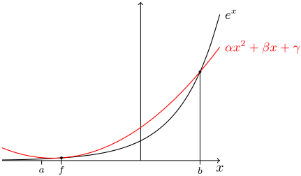
Theorem A.1 (Parabola Fitting). For a < b and b, z > 0, there exists α, β, γ that: αx2 + βx + γ ≥ exp(x) for all a ≤ x ≤ b, and zα + γ = (z exp(b) + b2 exp(-z/b))(z + b2 )-1 .
Proof. Parabola αx2+βx+γ that satisfies these requirements touches the exponential curve at one point (at x = f < b) and intersects it at another (at x = b), per Figure 1, thus:
This gives α, β, γ, in terms of f and b, hence: zα+γ = (((z+fb-b)(f-b-1)-b)ef +(f 2+z)eb )(b-f)-2 Minimizing with f occurs at f = -z b and gives the result.
Proof of Lemma 3.5. Assume WLOG that X has a mean of zero. We construct an upper bound for E [exp(sX)] by parabola over exp(sX). There exists a parabola defined by α, β, γ (Theorem A.1) and thus we expand: E [exp(sX)] ≤ E[αs2X2 + βsX + γ] = αs2 E[X2 ] + γ = αs2σ2 + γ
Proof of Lemma 3.6. Assume WLOG X has a mean of zero. We construct an upper bound for E [exp(-qX2 )] by parabola over exp(-qX2 ). For α, γ such that αX2 + γ ≥ exp(-qX2 ) for all a < X < b. If we define d = max(b, -a) we can choose γ = 1 and α = (exp(-qd2 ) - 1)d-2 (see figure 2) which results in:
Then because: exp(sχm) = ∏n-1 k=m exp ( sk (χk+1 - Xk+1)) E[exp(sχm)] =
by repeated application of the law of total expectation.
Since: E[Xk+1|χk+1 . . . χn] = χk+1 then χk+1 -Xk+1 is a random variable with a mean of zero bounded within width D, and it also has a variance given by:
Proof of Theorem 4.2. Applying Lemma 3.3:
by independence of the sampling between the strata. This is sufficient for Lemmas 3.7, and 3.5 to apply giving:
Proof of Theorem 4.3. To bound the sum of variances (weighted by arbitrary positive θi), consider the average square of samples about the strata means. Applying Lemma 3.3 gives:
Minimizing with respect to s, rearranging, and applying Lemma 3.2 gives result.
Proof of Theorem 4.4. We consider the weighted square error of the sample means:
P (∑ni=1 θi(µi - χi,mi )2 ≥ r) ≤ 1 - ∏ni=1 P (θi(µi - χi,mi )2 ≤ ri ) = 1∏ni=1 (1 - P (µi -χi,mi ≥ √ ri θi ) - P (χi,mi - µi ≥ √ ri θi )) such that ∑ ri = r, by independence of the sampling and probability complementarities. Applying Lemma 3.3 together with Lemmas 3.7, 3.4, gives: P (∑ni=1 θi(µi - χi,mi )2 ≥ r) ≤ 1 - ∏ni=1 (1-2 exp (- 2ri θiD2 i Ωni mi )) Choosing ri to minimize this expression gives: )-1
Proof of Theorem 4.5. By widening the bound of Equation (2) we get:
Completing the square gives for √∑ni=1 θiσ2 i gives:
Combining with Equation (3) with a union bound (Lemma 3.1) gives:
Which is a bound for the weighted sum variances in terms of the sample variances. Letting θi = 12 τ 2 i Ψni mi and combining with (1) with a union bound (Lemma 3.1), and then assigning r = t = y = p/3 and rewriting in terms of unbiased sample variance, gives the result.
Proof of Theorem 6.1. Squaring (4) and applying it specifically to the jth component of all the vectors gives:
Taking a series of union bounds (Lemma 3.1) over j gives us our result.
@inproceedings{ijcai2021p11,
  title     = {Approximating the Shapley Value Using Stratified Empirical Bernstein Sampling},
  author    = {Burgess, Mark A. and Chapman, Archie C.},
  booktitle = {Proceedings of the Thirtieth International Joint Conference on
               Artificial Intelligence, {IJCAI-21}},
  publisher = {International Joint Conferences on Artificial Intelligence Organization},
  editor    = {Zhi-Hua Zhou},
  pages     = {73--81},
  year      = {2021},
  month     = {8},
  note      = {Main Track},
  doi       = {10.24963/ijcai.2021/11},
  url       = {https://doi.org/10.24963/ijcai.2021/11},
}
TY - CPAPER TI - Approximating the Shapley Value Using Stratified Empirical Bernstein Sampling AU - Burgess, Mark A. AU - Chapman, Archie C. T2 - Proceedings of the Thirtieth International Joint Conference on Artificial Intelligence, IJCAI-21 PB - International Joint Conferences on Artificial Intelligence Organization PY - 2021 SP - 73 EP - 81 DO - 10.24963/ijcai.2021/11 UR - https://doi.org/10.24963/ijcai.2021/11 ER -Copied
Machine-readable versions of this paper, for tools and AI agents:





