
Online Portfolio Selection with Cardinality Constraint and Transaction Costs based on Contextual Bandit
Proceedings of the Twenty-Ninth International Joint Conference on Artificial Intelligence. Special Track on AI in FinTech. Pages 4682-4689.
https://doi.org/10.24963/ijcai.2020/646
Keywords
- Foundation for AI in FinTech: Reinforcement learning for FinTech
- AI for trading: General
- AI for trading: AI for portfolio analytics
- AI for trading: AI for strategic trading and strategy design
Abstract
Online portfolio selection (OLPS) is a fundamental and challenging problem in financial engineering, which faces two practical constraints during the real trading, i.e., cardinality constraint and non-zero transaction costs. In order to achieve greater feasibility in financial markets, in this paper, we propose a novel online portfolio selection method named LExp4.TCGP with theoretical guarantee of sublinear regret to address the OLPS problem with the two constraints. In addition, we incorporate side information into our method based on contextual bandit, which further improves the effectiveness of our method. Extensive experiments conducted on four representative real-world datasets demonstrate that our method significantly outperforms the state-of-the-art methods when cardinality constraint and non-zero transaction costs co-exist.
- [Auer et al., 2002] Peter Auer, Nicolo Cesa-Bianchi, Yoav Freund, and Robert E Schapire. The nonstochastic mul- tiarmed bandit problem. SIAM Journal on Computing, 32(1):48-77, 2002.
- [Blum and Kalai, 1999] Avrim Blum and Adam Kalai. Uni- versal portfolios with and without transaction costs. Ma- chine Learning, 35(3):193-205, 1999.
- [Boyd et al., 2011] Stephen Boyd, Neal Parikh, Eric Chu, Borja Peleato, Jonathan Eckstein, et al. Distributed op- timization and statistical learning via the alternating direc- tion method of multipliers. Foundations and Trends R in Machine learning, 3(1):1-122, 2011.
- Thomas M Cover and Erik Or- dentlich. Universal portfolios with side information. IEEE Transactions on Information Theory, 42(2):348- 363, 1996.
- Thomas M Cover. Universal portfolios. Math- ematical Finance, 1(1):1-29, 1991.
- [Das et al., 2013] Puja Das, Nicholas Johnson, and Arindam Banerjee. Online lazy updates for portfolio selection with transaction costs. In Twenty-Seventh AAAI Conference on Artificial Intelligence, 2013.
- [Das et al., 2014] Puja Das, Nicholas Johnson, and Arindam Banerjee. Online portfolio selection with group sparsity. In Twenty-Eighth AAAI Conference on Artificial Intelli- gence, 2014.
- [Duchi et al., 2008] John Duchi, Shai Shalev-Shwartz, Yoram Singer, and Tushar Chandra. Efficient projections onto the l 1-ball for learning in high dimensions. In Proceedings of the 25th International Conference on Machine Learning, pages 272-279, 2008.
- [Györfi and Vajda, 2008] László Györfi and István Vajda. Growth optimal investment with transaction costs. In In- ternational Conference on Algorithmic Learning Theory, pages 108-122, 2008.
- [Hakansson and Ziemba, 1995] Nils H Hakansson and William T Ziemba. Capital growth theory. Handbooks in operations research and management science, 9:65-86, 1995.
- [Hazan and Kale, 2015] Elad Hazan and Satyen Kale. An online portfolio selection algorithm with regret logarith- mic in price variation. Mathematical Finance, 25(2):288- 310, 2015.
- [Helmbold et al., 1997] David P Helmbold, Robert E Schapire, Yoram Singer, and Manfred K Warmuth. A comparison of new and old algorithms for a mixture estimation problem. Machine Learning, 27(1):97-119, 1997.
- [Helmbold et al., 1998] David P Helmbold, Robert E Schapire, Yoram Singer, and Manfred K Warmuth. On-line portfolio selection using multiplicative updates. Mathematical Finance, 8(4):325-347, 1998.
- [Huang et al., 2015] Dingjiang Huang, Yan Zhu, Bin Li, Shuigeng Zhou, and Steven CH Hoi. Semi-universal port- folios with transaction costs. In Twenty-Fourth Interna- tional Joint Conference on Artificial Intelligence, 2015. IJCAI
- [Huang et al., 2016] Dingjiang Huang, Junlong Zhou, Bin Li, Steven CH Hoi, and Shuigeng Zhou. Robust median re- version strategy for online portfolio selection. IEEE Trans- actions on Knowledge and Data Engineering, 28(9):2480- 2493, 2016.
- [Ito et al., 2018] Shinji Ito, Daisuke Hatano, Sumita Hanna, Akihiro Yabe, Takuro Fukunaga, Naonori Kakimura, and Ken-Ichi Kawarabayashi. Regret bounds for online pport- folio selection with a cardinality constraint. In Advances in Neural Information Processing Systems, pages 10588- 10597, 2018.
- [Li and Hoi, 2014] Bin Li and Steven CH Hoi. Online port- folio selection: A survey. ACM Computing Surveys (CSUR), 46(3):35, 2014.
- [Li et al., 2012] Bin Li, Peilin Zhao, Steven CH Hoi, and Vivekanand Gopalkrishnan. Pamr: Passive aggressive mean reversion strategy for portfolio selection. Machine Learning, 87(2):221-258, 2012.
- [Li et al., 2018] Bin Li, Jialei Wang, Dingjiang Huang, and Steven CH Hoi. Transaction cost optimization for online portfolio selection. Quantitative Finance, 18(8):1411- 1424, 2018.
- [Liu et al., 2016] Yong-Jun Liu, Wei-Guo Zhang, and Jun- Bo Wang. Multi-period cardinality constrained portfolio selection models with interval coefficients. Annals of Op- erations Research, 244(2):545-569, 2016.
- [Mishra et al., 2014] Sudhansu Kumar Mishra, Ganapati Panda, and Ritanjali Majhi. A comparative performance assessment of a set of multiobjective algorithms for con- strained portfolio assets selection. Swarm and Evolution- ary Computation, 16:38-51, 2014.
- [Moeini, 2019] Mahdi Moeini. Orthogonal bandit learning for portfolio selection under cardinality constraint. In In- ternational Conference on Computational Science and Its Applications, pages 232-248, 2019.
- [Shen et al., 2014] Weiwei Shen, Jun Wang, and Shiqian Ma. Doubly regularized portfolio with risk minimization. In Twenty-Eighth AAAI Conference on Artificial Intelligence, 2014.
- [Syrgkanis et al., 2016] Vasilis Syrgkanis, Akshay Krishna- murthy, and Robert Schapire. Efficient algorithms for ad- versarial contextual learning. In International Conference on Machine Learning, pages 2159-2168, 2016.
- [Wei and Luo, 2018] ChenYu Wei and Haipeng Luo. More adaptive algorithms for adversarial bandits. In Conference On Learning Theory, pages 1263-1291, 2018.
References were extracted automatically from the PDF and may contain errors.
Full text extracted automatically from the PDF; figures, tables and equations may differ. The PDF is the version of record.
1 Introduction
Online portfolio selection (OLPS), which aims to construct a portfolio to optimize the allocation of wealth across a set of assets for the highest return, has been extensively investigated in recent years [Li and Hoi, 2014]. Most of the proposed methods [Li et al., 2012; Huang et al., 2016], however, overlooked two constraints in the real trade practice, i.e., cardinality constraint and non-zero transaction costs.
On one hand, the cardinality constraint problem is one of the big challenges in OLPS, which refers to limiting the number of assets, instead of including all assets in an efficient portfolio. As far as investors are concerned, cardinality constraint enables them to limit the complexity of a portfolio and reduce managerial concerns. However, Ito et al. [2018] prove that OLPS with cardinality constraint is an NPcomplete problem. The number of cardinality constrained assets combinations grows exponentially with the number of assets. Hence, it is computationally infeasible to construct portfolios of all combinations and choose the optimal one.
On the other hand, how to constrain the non-zero transaction costs is an important open issue in OLPS. Transaction cost is one central friction in real-world financial markets. Every time when an investor changes his/her portfolio, the investor needs to pay a certain transaction cost. However, most state-of-the-art OLPS methods overlooked transaction cost [Hazan and Kale, 2015; Huang et al., 2016; Ito et al., 2018], which might lead to overtrading with hefty transaction costs in practice, and even losing profits.
∗Corresponding Author
Based on the above analysis, we propose a novel method called LExp4.TCGP to address the OLPS problem with the two constraints, i.e., cardinality constraint and non-zero transaction costs. LExp4.TCGP first exploits side information of assets to sequentially generate a probability distribution over the cardinality constrained assets combinations. Then based on the probability distribution and a lazy sample mechanism, our method selects the nearly-optimal assets combination based on our proposed contextual bandit framework. Finally, our method allocates wealth of the selected assets combination with the trade-off between the expected return and transaction costs.
Specifically, we give the details of how LExp4.TCGP deals with the two constraints. Firstly, for cardinality constraint, we model the assets combination selection into a bandit framework. To further improve the effectiveness of the selection, we exploit side information which can provide hints that one or a set of assets are likely to be superior to the others [Cover and Ordentlich, 1996] and propose a contextual bandit algorithm. To the best of our knowledge, our method is the first bandit-based OLPS method considering the side information. Secondly, for constraining non-zero transaction costs, we develop two mechanisms to reduce trading volumes in the complex process consisting of assets combination selection and wealth allocation, which is equivalent to minimizing the incurred transaction costs. In assets combination selection, the portfolio changes whenever selling or buying any assets. Such behavior consumes much transaction cost, hence we devise a lazy sample mechanism to reduce the changes of the selected assets combination. In wealth allocation, each adjustment of weights consumes transaction cost, so we develop a new algorithm named TCGP to minimize the difference between two consecutive allocations. In general, our model not only satisfies two constraints, but also achieves sublinear regret, which is a strong theoretical performance guarantee to address the OLPS problem.
To sum up, our main contributions are as follows: (1) We propose a novel LExp4.TCGP method to achieve greater feasibility in financial markets; (2) We incorporate side information to improve the effectiveness of the proposed method; (3) We have rigorously proven that LExp4.TCGP method achieves sublinear regret, which indicates that our method has a strong theoretical performance guarantee; and (4) We have conducted extensive experiments on four real-world datasets, which empirically demonstrate that our method significantly outperforms the state-of-the-art methods when cardinality constraint and non-zero transaction costs co-exist.
2 RelatedWork
OLPS has been studied in different disciplines, including finance, statistics, machine learning, and optimization. Although the need for considering real constraints has been mentioned [Li and Hoi, 2014], only a few studies deal with the real constraints.
The cardinality constrained OLPS problem has been studied by several researchers, whose solutions can be classified into three categories. The first category uses a repair mechanism to delete the assets with smaller weights [Mishra et al., 2014; Liu et al., 2016], which lacks theoretical performance guarantee and performs poorly when weights are close to each other. The second category adds a sparsity regularization term to allocate weight concentrating on a few assets. Das et al. [2014] added a surrogate group-sparse constraint to the OLPS model, which has a motivation similar to cardinality constraint, but they did not consider any constraint about cardinality directly. The third category is to construct a multi-armed bandit framework to select an assets combination with cardinality constraint. Ito et al. [2018] proposed two algorithms in Full-feedback setting and Bandit-feedback setting to select an assets combination and calculate the portfolios of all assets combinations and that of the selected assets combination respectively. Moeini [2019] combined orthogonal bandit learning with a kernel search heuristic. However, all of them do not consider the side information, with which the OLPS models can become more effective in financial markets.
Targeting the OLPS problem, the methods of considering transaction costs are mainly divided into three categories. The first category focuses on occasional rebalancing. Helmbold et al.[1998] considered a semi constant rebalanced portfolio (SCRP) method and Huang et al. [2015] proposed a semiuniversal portfolio (SUP) method, which rebalances only in some periods. The second one is extended from universal portfolio (UP) [Cover, 1991], which utilizes UP formulation as a moving target portfolio [Blum and Kalai, 1999] and then rebalances the portfolio in each investment period. The last category modifies the objective function via adding a regularization term [Das et al., 2013; Shen et al., 2014; Li et al., 2018]. However, all of the above methods are not applicable in the case of cardinality constraint, because in the cardinality constrained OLPS problem, we need to consider the difference not only between two consecutive allocations but also between two consecutive assets combinations.
In a word, none of the existing work in OLPS has attempted to investigate two real constraints with theoretical performance guarantee in their algorithms.
3 Problem Settings
Consider a financial market with n assets, we invest our wealth in the market for a sequence of T trading periods. In each trading period, the price relatives of the assets are denoted as a vector r = (r1, r2, ..., rn), where ri is the next period's opening price of the asset i divided by its opening price in the current period, which is bounded in a closed interval [C1, C2] (C1 and C2 are constants satisfying 0 < C1 ≤ C2).
In general, some assumptions bellow are widely adopted in OLPS problem [Li and Hoi, 2014], which are also followed in our paper: (1) No margin/short: margin purchase and short sale are not allowed; (2) Unlimited market liquidity: one can buy and sell any quantity of any asset in its closing prices; and (3) Zero impact cost: market behaviors are not impacted by any OLPS method.
Online Portfolio SelectionProblem. Aportfolio is defined by a weight vector w = (w1, w2, ..., wn) satisfying the constraint that every weight wi is non-negetive and the sum of all the weights equals one, i.e., w ∈ {w|w ≥ 0,w⊤1 = 1}. The element i of w indicates the proportion of wealth allocated to the asset i. Let wt denote the weight of portfolio for a period t. After T periods, an OLPS strategy increases the initial wealth A0 by a factor of ∏Tt=1 (w⊤ t rt), namely, the final cumulative wealth after T periods is AT (w) = A0 ∏Tt=1 (w⊤ t rt). For the sake of simplicity, we set A0 = 1. Since the model assumes multi-period investment, we define the logarithmic cumulative wealth according to the capital growth theory [Hakansson and Ziemba, 1995] as log AT (w) = ∑Tt=1 log(w⊤ t rt).
Cardinality Constraint. The combination of assets is restricted to a set of available combinations S ⊆ [n]. For an assets combination S ∈ S, ∆S is the set of portfolios which satisfies ∆S = {w|w ≥ 0, w⊤1 = 1, supp(w) ⊆ S}, where supp(w) = {i ∈ [n]|wi ̸= 0}. Ito et al. [2018] define a special form of S with cardinality constraint, Sk := {S ⊆ [n]||S| ≤ k} for some k ≤ n. Note that when S = Sn, the problem coincides with the standard online portfolio selection problem, and the problem even turns into the single asset selection problem when S = S1.
TransactionCosts. Following the proportional transaction costs model [Gy¨orfi and Vajda, 2008], we can get a new logarithmic cumulative wealth with non-zero transaction costs:
where ct-1 denotes the transaction costs factor as the ratio of the net wealth after transaction costs incurred. Then we have:
where γ is the transaction cost rate (Note that we equalize the rates of purchases and sales, which is widely adopted by related research [Gy¨orfi and Vajda, 2008; Li et al., 2018]) and the renormalized portfolio weight ˆwt-1 = wt-1◦rt-1 w⊤ t-1 rt-1 (the symbol ◦ denotes the Hadamard product). Moreover, Li et al. [2018] gave the bound of ct-1 as 1-γ 1-γ+γ‖ ˆwt-1-wt‖1 ≤
ct-1 ≤ 1+γ 1+γ+γ‖ ˆwt-1-wt‖1 , which is inversely related to ‖ˆwt-1 -wt‖1 , namely, the smaller the ℓ1 term, the larger the value of ct-1.
Definition of Regret. Let fT (w∗ ) denote the optimal fix (non-shifting) portfolio in hindsight for T periods, namely,
∑Tt=1 ft(wS ). In our setting, we
adopt the formula of ft(wS ) as:
where wS ∈ ∆S , λ ≤ 0 is a trade-off parameter to balance the expected return and trading volume. In particular, the regret after T-periods is defined as:
4 Methodology
To address the OLPS problem with cardinality constraint and transaction costs, we propose the LExp4.TCGP algorithm, which sequentially selects assets combination (LExp4) and allocates wealth of the selected combination (TCGP) until the end of trading periods. In this section, we first introduce the selection and allocation parts respectively, then give the entire algorithm and finally give the theoretical analysis.
4.1 Assets Combination Selection: Lazy Exp4 (LExp4) Algorithm
We model the assets combination selection problem as a multi-arm bandit problem. The main advantage comes from the fact that the investors need not to observe all the assets; rather, they only need to focus on the assets in the selected combination. So we need not to always update wS t for all S ∈ Sk. Regarding the OLPS problem, it is hard to assume that the rewards are truly randomly generated, especially when it comes to competitive financial scenarios. Therefore, we propose an adversarial contextual bandit algorithm LExp4 based on Exp4 algorithm [Auer et al., 2002] with a lazy sample mechanism for selecting assets combination to reduce the changes of the selected combination.
Consider there are some experts who sequentially give their advices of which assets combination is likely to be superior to others. Note that the expert does not mean a real person, in our paper, it is an online policy. The goal of LExp4 algorithm is to combine the experts' advices by an expert trust vector q which measures experts' credibilities, so that its selected assets combination is close to the optimal combination in hindsight. We use ξit to denote the |Sk|-dimensional expert's advice vector, which represents a probability distribution over the assets combinations which are recommended by expert i on period t. Specifically, ξit ∈ [0, 1]|Sk| and Σ|Sk | j=1 ξ i t,j = 1.
There are many ways to construct the sequence of experts' advices. Most of the existing contextual bandit methods, however, adopted offline policies [Syrgkanis et al., 2016;
Algorithm 1 Generate Experts' Advices (GEA)
Input: θt ∈ R(m-1)×d , xt ∈ Rn×d .
Output: ξt.
- 1: for i = 1, ...,m-1 do
- 2: Convert xt into xit .
- 3: Predict yt,a = θit⊤xit,a , where a = 1, ..., n.
- 4: for each S ∈ Sk do
- 5: ¯yt,S = mean(yt,a), where a ∈ S.
- 6: end for
- 7: ξit,S = 1 argsort(¯yt,S) , where S ∈ Sk.
- 8: Normalize ξit .
- 9: end for
Wei and Luo, 2018], which are not applicable to the dynamic OLPS issue. Therefore, we propose a novel online policy to generate experts' advices (see Algorithm 1). Let xt ∈ Rn×d be the side information of all assets available in period t. We assume each expert has a binary vector zi ∈ Rd and coefficients θi ∈ Rd of side information, where i is the expert's index. In particular, the binary vector specifies whether a particular dimension of side information participates in the prediction, which is generated based on a binary coding of the expert's index. Experts' advices are designed as follows. In period t, each expert first converts xt into xit associated with the binary vector zi and predicts all assets' rewards. Then the expert sorts the assets combinations by their average predict rewards. Finally the expert uses the reciprocal ranks as the probabilities of assets combinations and normalizes the total probabilities to one. Beside, we include a uniform expert ξ, which always assigns uniform probabilities to all assets combinations. Therefore, there are totally m = 2d experts.
After generating the m experts' advices ξ1t , ..., ξmt , the LExp4 algorithm lazily samples an assets combination St ∈ Sk based on the experts' comprehensive recommendation. The experts' comprehensive recommendation is a sampling distribution pt of all combinations with an exploitation and exploration trade-off calculated as:
where β ∈ (0, 1) is the exploration parameter.
Specifically, the lazy sample mechanismmeans sample assets combination occasionally. The total trading periods are divided into several segments, and in each segment the LExp4 algorithm only samples the combination once; but the rewards and the experts' adviecs in each segment are still accumulated into the expert trust vector q.
4.2 Wealth Allocation: Transaction Costs-aware Gradient Projection (TCGP) Algorithm
Following the definition in problem settings, we can give the objective function of weight wt at period t, which allows us Algorithm 2 Transaction Costs-aware Gradient Projection (TCGP)
2: ADMM iterations
- 3: Continue until stopping criteria are satisfied.
- 4: Output wt,St =wt.
to control the transaction volume, as follows:
The purpose of the first term is to maximize logarithmic wealth based on Exponential Gradient-type [Helmbold et al., 1998], which implies that the portfolio vector itself encapsulates the necessary information from the previous price relative rt-1. The second term is the ℓ1 penalty, which is used to control transactions volume leading to reduce transaction costs. The third term denotes a regularization term, where we use ℓ2 norm regularization, which is same as gradient projection algorithm [Helmbold et al., 1997].
Since there is an ℓ1 term in our objective function, we propose a TCGP algorithm based on alternating direction method of multipliers (ADMM) algorithm [Boyd et al., 2011] to solve Eq.(6). By decoupling ℓ1 term and replacing the log term with its first order Taylor expansion around wt-1, the augmented Lagrangian for the above problem becomes,
where z = w - ˆwt-1, u = 1ρ y is the scaled dual variable, and y is the dual variable. Using the scaled dual variable, TCGP algorithm consists of the iterations for solving wt (see Algorithm 2).
The projection to the simplex ∏p∈∆St is carried out as in [Duchi et al., 2008]. The function Sλ/ρ denotes the soft thresholding operator and the stopping criteria are based on the primal and dual residuals [Boyd et al., 2011].
4.3 LExp4.TCGP Algorithm
In each trading period, LExp4.TCGP consists of three steps: (1) it selects assets combination; (2) it allocates wealth of the selected combination; (3) it observes price relatives r and updates θ and q. The LExp4.TCGP algorithm is summarized in Algorithm 3.
Algorithm 3 LExp4.TCGP
Input: T periods, n assets, m experts, cardinality k, the segment length κ, the exploration parameter β.
- 1: Initial θ1 = 0, q1 = 1.
- 2: for each t = 1, ..., T do
- 3: Observe side information of all assets xt ∈ Rn×d .
- 4: Get mexperts' advices ξ1t , ξ2t , ..., ξmt =GEA(θt, xt).
- 5: if t ≡ 0 (mod κ) then
- 6: Draw assets combination St randomly according to the sampling distribution pt by Eq.(5).
- 7: else
- 8: St = St-1
- 9: end if
- 11: Observe price relatives rt.
- 12: // Update θ.
- 13: for i = 1, ..., m - 1 do
- 14: Convert xt into xit .
- 16: end for
- 17: // Update q.
- 18: for each S ∈ Sk do
- 20: end for
- 21: for i = 1, ..., m do
- 22: ˆ ν i t = ξit⊤ ˆyt.
- 23: qi t+1 = qi t exp(αˆ vi t /|Sk|).
- 24: end for
- 25: end for
4.4 Analysis of Regret
The theoretical performance of OLPS methods is measured by regret RT . First of all, we derive the regret upper bound of our method in Theorem 1.
Theorem 1. For any T > 0, let w∗ ∈ ∆S∗ be the optimal portfolio obtained from max S∈S,w∈∆S ∑Tt=1 ft(S,w). Let the sequence of wt be defined as the output in LExp4.TCGP. Suppose ‖ˆw-w‖1 ≤ L, ∀w, ˆw ∈ ∆S . For any ϵ > 0 and 0 < q < 1, the regret of LExp4.TCGP can be bounded as:
The complete proof of Theorem 1 will be available in a longer version of the paper.
Next, we theoretically analyze the regret of our method compared with that of other methods in three typical cases:
(1) Single asset selection (S = S1): We compare with two methods, i.e., Full-feedback and Bandit-feedback [Ito et al., 2018] to discuss the performance towards finding the optimal assets combination. In Table 1, if there is no transaction cost (λ = 0), all methods achieve O(√T). Full-feedback performs the best. When m ≤ n, our method has a better performance; otherwise, Bandit-feedback performs better. With the non-zero transaction costs (λ > 0), Full-feedback and Bandit-feedback achieve O(T) which is larger than ours.
(2) Standard portfolio selection (S = Sn): We compare with OLU [Das et al., 2013] which only considers the transaction costs but overlooks cardinality constraint. The regret of our method and OLU are both O(√nT ) + λO(√T ), but OLU's regret formulation uses an impractical termwt-1 which does not follow the general trading principle [Li et al., 2018]. Instead, we use the renormalized portfolio weight ˆwt-1. Thus OLU's regret bound has a gap between ˆwt-1 and wt-1, and our method has a smaller regret bound than OLU.
(3) Cardinality constrained portfolio selection (S = Sk): As highlighted in Theorem 1, our LExp4.TCGP achieves a sublinear regret O(√T ) after T trading periods. For an online learning algorithm, a sublinear regret upper bound is vital, as it indicates the average number of suboptimal portfolio that makes vanishes rapidly over time.
In addition, RR-DE [Liu et al., 2016] and NS-MOPSO [Mishra et al., 2014] can address OLPS problem with cardinality constraint, but little is known about their regret bounds.
5 Experiments
In this section, we present the extensive experiments conducted on four representative real-world datasets.
| Constraints | Single Asset (S = S1) | Cardinality Constraint (S = Sk) | Standard (S = SN ) |
|---|---|---|---|
| LExp4.TCEG | O(√nT logm) +λO(√T ) | O(√T|Sk| logm) +λO(√T ) | O(√nT) +λO(√T ) |
| Full-feedback | O(√T logn) +λO(T ) | O(√T log |Sk|) +λO(T ) | O(√T logn) +λO(T ) |
| Bandit-feedback | O(√nT logn) +λO(T ) | O(√T|Sk| logn) +λO(T ) | O(√T logn) +λO(T ) |
| OLU | - | - | O(√nT ) +λO(√T ) |
n denotes the number of stocks; T is the number of trading periods; m denotes the number of experts; Sk denotes assets combinations with k cardinality constraint.
| Dataset | Region | Time frame | # Days | # Assets |
|---|---|---|---|---|
| NYSE | US | 06/03/1962 - 12/31/1984 | 1,259 | 36 |
| TSE | CA | 01/04/1994 - 12/31/1998 | 544 | 88 |
| DJIA | US | 01/14/2001 - 01/14/2003 | 507 | 30 |
| SP500 | US | 02/11/2013 - 02/07/2018 | 1,355 | 500 |
Table 2: Summary of the four datasets
5.1 Experimental Settings
Data Collection. The experiments are conducted on four public datasets: the NYSE, TSE, DJIA, and SP500 datasets, which are summarized in Table 2. In particular, the NYSE dataset [Cover, 1991] consists of 36 stocks from the New York Stock Exchange. The TES [Li et al., 2012] dataset includes 88 stocks of Canada market from the Toronto Stock Exchange (TSE). The DJIA dataset is a collection of Dow Jones 30 composite stocks [Huang et al., 2016]. The SP500 dataset contains 500 stocks of the S&P 500 index 1 .
Comparisonmethods. The representative and state-of-theart methods compared in our experiments can be categorized
1 https://www.kaggle.com/camnugent/sandp500
| Methods | NYSE | TSE | DJIA | SP500 | ||||||||
|---|---|---|---|---|---|---|---|---|---|---|---|---|
| 1 | 5 | n | 1 | 5 | n | 1 | 5 | n | 1 | 5 | n | |
| NS-MOPSO | 7.89 | 10.91 | 11.81 | 0.57 | 0.79 | 0.71 | 1.00 | 1.31 | 1.64 | 0.96 | 1.09 | 1.28 |
| Full-feedback1 | 3.31E-23 | - | 2.21E-03 | 1.96E-03 | - | 1.41E-01 | 3.49E-06 | - | 0.08 | 1.16E-05 | - | 1.04 |
| Bandit-feedback | 8.49E-23 | 1.01E-20 | 2.21E-03 | 6.34E-03 | 0.01 | 0.14 | 1.38E-06 | 2.08E-05 | 0.08 | 6.43E-06 | 7.01E-06 | 1.04 |
| OLU2 | - | - | 29.88 | - | - | 0.81 | - | - | 1.58 | - | - | 1.87 |
| DRP2 | - | - | 28.39 | - | - | 0.79 | - | - | 1.64 | - | - | 1.93 |
| TCO2 | - | - | 2.31E+06 | - | - | 0.12 | - | - | 0.92 | - | - | 2.36 |
| RR-DE | 5.44 | 5.40 | 5.06 | 0.84 | 0.69 | 0.73 | 1.43 | 1.18 | 1.62 | 0.67 | 1.80 | 1.14 |
| LExp4.TCGP | 13.01 | 26.95 | 30.61 | 0.93 | 1.01 | 0.82 | 2.10 | 1.96 | 1.69 | 1.88 | 1.97 | 2.40 |
- 1 Due to too many assets combinations to be calculated, the Full-feedback method cannot run under the S = S5 within a tolerable time.
- 2 OLU, DRP, TCO methods cannot address the cardinality constraint problem, so they can only be compared with the results in standard portfolio selection (S = Sn).
Table 3: Cumulative wealth achieved by various methods with different cardinality constraints (γ = 0.005, k = 1, 5, n).
into three groups:
(1) OLPS with Cardinality Constraint: NS-MOPSO [Mishra et al., 2014] , Full-feedback [Ito et al., 2018], and Bandit-feedback [Ito et al., 2018].
- OLPS with Transaction Costs: OLU [Das et al., 2013], TCO [Li et al., 2018], and DRP [Shen et al., 2014].
- OLPS with Cardinality Constraint and Transaction Costs: RR-DE [Liu et al., 2016].
Among them, NS-MOPSO is a single-period OLPS method, so we apply the interval programming approach [Liu et al., 2016] to amend it to be a multi-period method.
Experiments Setups and Metrics. We collect the assets' side information of the above datasets. Each asset is associated with an 8-dimensional feature vector, which include: the average price relatives of last 1, 3, 6, 12 days and the average trading volume of last 1, 3, 6, 12 days (Note that the average trading volume are only available on the SP500 dataset).
Regarding parameter settings, we set the trade-off parameter λ = 10×γ (γ is the transaction cost rate) and the parameter for the augmentation term ρ = 0.1, which are empirically effective. In addition, we set the parameters β, η, κ according to Theorem 1. We use the parameter settings recommended in the relevant studies for other comparison methods.
We use the standard metrics in finance [Li et al., 2012] to measure the performance of the OLPS methods: (1) Cumulative wealth (CW); (2) Turnover (TU); (3) Maximum drawdown (MD); (4) Volatility (VO); (5) Sharpe ratio (SR); (6) Camer ratio (CR). Among them, CW is the most common metric to primarily compare different trading strategies. TU is a measure of trading volume in a time period, which evaluates whether the strategy can constrain the transaction costs. In general, the higher the values of the CW, and the lower TU, the better the performance of the compared algorithm. For some process-dependent investors, it is important to evaluate risk and risk-adjusted return of portfolios. One common way to achieve this is to use VO to measure the volatility risk and SR to evaluate the risk-adjusted return concerning the volatility risk. Another way focuses on drawdown which measures the decline from a historical peak in the cumulative wealth achieved by a financial trading strategy. So we adopts MD to measure downside risk and CR to measure the return relative to the drawdown risk of a portfolio. Generally speaking, the smaller the VO and MD, the more risk tolerable the financial trading strategy. Higher SR and CR indicate better performance of a trading strategy concerning the volatility risk and the drawdown risk. Note that all metrics are adjusted by transaction costs following the OLPS framework [Li et al., 2018].
5.2 Experimental Results
Evaluation with different cardinality constraints. We backtest three reasonable cardinality constraints representing 3 cases: single asset selection (k = 1), standard portfolio selection (k = n), and cardinality constrained portfolio selection (k = 5). Table 3 presents the CW achieved in the above three cases and the best result in each column is highlighted in bold. Note that Full-feedback and Bandit-feedback are excluded from the analysis below, because they trade overly and their profits are almost consumed by transaction costs.
In Table 3, LExp4.TCGP achives the highest CW with different cardinality constraints. (1) In single asset selection, our method outperforms NS-MOPSO and RR-DE by 10.7% and 180.6% respectively, because LExp4 plays an important role in our method to select the nearly-optimal asset; (2) In standard portfolio selection, our method outperforms all of the state-of-the-art methods by an average of 90.6%, ranging from 1.2% to 583.3% (except TCO on the NYSE dataset), because TCGP helps LExp4.TCGP to allocate wealth more effectively. TCO performs extremely better than our method only on the NYSE dataset, because it overly exploits the old and (weak-form) inefficient the market in the NYSE dataset and gains huge profit according to Li et al. [2018]'s analysis. In contrast, TCO performs poorly on all the other three datasets; (3) In cardinality constrained portfolio selection, our method performs the best with an average improvement 98.8%, ranging from 27.9% to 346.1%, because of the superiority of both LExp4 and TCGP.
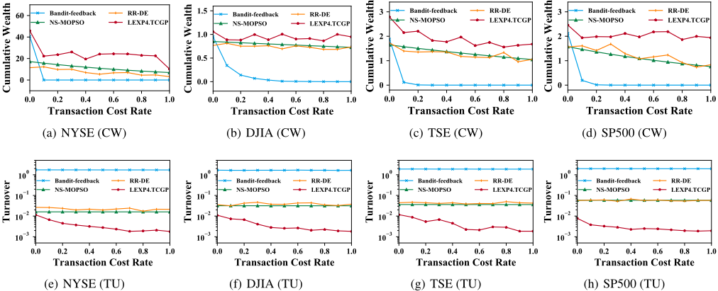
Evaluation with varying transaction cost rates. To better illustrate the effectiveness of our method with transaction cost, we compare the state-of-the-art methods in terms of CW. Figure 1 plots the CW and TU with varying transaction cost rates. We can draw three conclusions from Figure 1. (1) On all levels of transaction cost rates, LExp4.TCGP always achieves the highest CW, because it has the lowest TU, which can prevent profit from being robbed by transaction costs; (2) LExp4.TCGP's TU consistently decreases to almost zero when the transaction cost rate increases, which illustrates that LExp4.TCGP can trade off between the transaction cost rate and turnover; (3) The CW of LExp4.TCGP is higher than Bandit-feedback with zero transaction cost rate, because our method also considers side information which the Bandit-feedback overlooks. This demonstrates that leveraging side information can improve the effectiveness of our method.
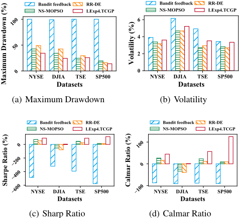
Evaluation of risk and risk-adjusted return. At last, we evaluate the risk in terms of MD and VO, and the riskadjusted return in terms of SR and CR. Figure 2 shows the results on all four datasets. In terms of MD, our method performs the best of all methods. In terms of VO, our method has lower risk than Bandit-feedback but higher risk than NSMOPSO and RR-DE methods (Figure 2 (b)), because high returns are usually accompanied by high risks. To further evaluate the trade-off of return and risk, we examine the riskadjusted return in terms of SR and CR. The results in Figure 2 (c) (d) show that our method performs the best, indicating the outstanding ability in balancing return and risk.
6 Conclusions
In this paper, we propose a novel method called LExp4.TCGP to address the OLPS problem with cardinality constraint and transaction costs. Extensive experiments show that our method can achieve satisfactory performance. In the future, we plan to extend our work into three potentially directions. The first direction is to consider more side information related to the financial market (e.g., coronavirus). The second direction is to extend our model to a risk-sensitive one. The third direction is to further reduce the time complexity of our method.
Acknowledgments
This work was supported in part by the National Key R&D Program of China (No. 2018YFB1403001).
@inproceedings{ijcai2020p646,
  title     = {Online Portfolio Selection with Cardinality Constraint and Transaction Costs based on Contextual Bandit},
  author    = {Zhu, Mengying and Zheng, Xiaolin and Wang, Yan and Liang, Qianqiao and Zhang, Wenfang},
  booktitle = {Proceedings of the Twenty-Ninth International Joint Conference on
               Artificial Intelligence, {IJCAI-20}},
  publisher = {International Joint Conferences on Artificial Intelligence Organization},
  editor    = {Christian Bessiere},
  pages     = {4682--4689},
  year      = {2020},
  month     = {7},
  note      = {Special Track on AI in FinTech},
  doi       = {10.24963/ijcai.2020/646},
  url       = {https://doi.org/10.24963/ijcai.2020/646},
}
TY - CPAPER TI - Online Portfolio Selection with Cardinality Constraint and Transaction Costs based on Contextual Bandit AU - Zhu, Mengying AU - Zheng, Xiaolin AU - Wang, Yan AU - Liang, Qianqiao AU - Zhang, Wenfang T2 - Proceedings of the Twenty-Ninth International Joint Conference on Artificial Intelligence, IJCAI-20 PB - International Joint Conferences on Artificial Intelligence Organization PY - 2020 SP - 4682 EP - 4689 DO - 10.24963/ijcai.2020/646 UR - https://doi.org/10.24963/ijcai.2020/646 ER -Copied
Machine-readable versions of this paper, for tools and AI agents:





