
Bridging Cross-Tasks Gap for Cognitive Assessment via Fine-Grained Domain Adaptation
Proceedings of the Twenty-Ninth International Joint Conference on Artificial Intelligence. Special track on AI for CompSust and Human well-being. Pages 4330-4337.
https://doi.org/10.24963/ijcai.2020/597
Keywords
- Machine Learning: Transfer, Adaptation, Multi-task Learning
- Humans and AI: Cognitive Modeling
- Humans and AI: Cognitive Systems
- Humans and AI: Human-Computer Interaction
Abstract
Discriminating pathologic cognitive decline from the expected decline of normal aging is an important research topic for elderly care and health monitoring. However, most cognitive assessment methods only work when data distributions of the training set and testing set are consistent. Enabling existing cognitive assessment models to adapt to the data in new cognitive assessment tasks is a significant challenge. In this paper, we propose a novel domain adaptation method, namely the Fine-Grained Adaptation Random Forest (FAT), to bridge the cognitive assessment gap when the data distribution is changed. FAT is composed of two essential parts 1) information gain based model evaluation strategy (IGME) and 2) domain adaptation tree growing mechanism (DATG). IGME is used to evaluate every individual tree, and DATG is used to transfer the source model to the target domain. To evaluate the performance of FAT, we conduct experiments in real clinical environments. Experimental results demonstrate that FAT is significantly more accurate and efficient compared with other state-of-the-art methods.
- [Banerjee et al., 2018] Imon Banerjee, Alexis Crawley, Mythili Bhethanabotla, Heike E Daldrup-Link, and Daniel L Rubin. Transfer learning on fused multiparamet- ric mr images for classifying histopathological subtypes of rhabdomyosarcoma. Computerized Medical Imaging and Graphics, 65:167-175, 2018.
- [Chen et al., 2018] Yiqiang Chen, Chunyu Hu, Bin Hu, Lisha Hu, Han Yu, and Chunyan Miao. Inferring cog- nitive wellness from motor patterns. IEEE Transactions on Knowledge and Data Engineering, 30(12):2340-2353, 2018.
- [Gao et al., 2020] Fei Gao, Hyunsoo Yoon, Teresa Wu, and Xianghua Chu. A feature transfer enabled multi-task deep learning model on medical imaging. Expert Systems with Applications, 143:112957, 2020.
- [Garre-Olmo et al., 2017] Josep Garre-Olmo, Marcos Faúndez-Zanuy, Karmele López-de Ipiña, Laia Calvó- Perxas, and Oriol Turró-Garriga. Kinematic and pressure features of handwriting and drawing: preliminary re- sults between patients with mild cognitive impairment, alzheimer disease and healthy controls. Current Alzheimer research, 14(9):960-968, 2017.
- [Gong et al., 2012] Boqing Gong, Yuan Shi, Fei Sha, and Kristen Grauman. Geodesic flow kernel for unsupervised domain adaptation. pages 2066-2073, 2012.
- [Hu et al., 2018] Chunyu Hu, Yiqiang Chen, Xiaohui Peng, Han Yu, Chenlong Gao, and Lisha Hu. A novel feature in- cremental learning method for sensor-based activity recog- nition. IEEE Transactions on Knowledge and Data Engi- neering, 31(6):1038-1050, 2018.
- [Kermany et al., 2018] Daniel S Kermany, Michael Gold- baum, Wenjia Cai, Carolina CS Valentim, Huiying Liang, Sally L Baxter, Alex McKeown, Ge Yang, Xiaokang Wu, Fangbing Yan, et al. Identifying medical diagnoses and treatable diseases by image-based deep learning. Cell, 172(5):1122-1131, 2018.
- [Khatami et al., 2018] Amin Khatami, Morteza Babaie, Hamid R Tizhoosh, Abbas Khosravi, Thanh Nguyen, and Saeid Nahavandi. A sequential search-space shrinking us- ing cnn transfer learning and a radon projection pool for medical image retrieval. Expert Systems with Application- s, 100:224-233, 2018.
- [Long et al., 2018] Mingsheng Long, Yue Cao, Zhangjie Cao, Jianmin Wang, and Michael I Jordan. Transfer- able representation learning with deep adaptation network- s. IEEE transactions on pattern analysis and machine in- telligence, 41(12):3071-3085, 2018.
- [Mathiowetz et al., 1985] Virgil G Mathiowetz, Gloria Vol- land, Nancy Kashman, and Karen Weber. Adult norms for the box and block test of manual dexterity. American Journal of Occupational Therapy, 39(6):386-391, 1985.
- [Montero-Odasso et al., 2009] Manuel Montero-Odasso, Howard Bergman, Natalie A Phillips, Chek H Wong, Nadia Sourial, and Howard Chertkow. Dual-tasking and gait in people with mild cognitive impairment. the effect of working memory. BMC geriatrics, 9(1):41, 2009.
- [Organization and others, 2017] World Health Organization et al. Global action plan on the public health response to dementia 2017-2025. 2017.
- [Pan and Yang, 2010] Sinno Jialin Pan and Qiang Yang. A survey on transfer learning. IEEE Transactions on Knowl- edge and Data Engineering, 22(10):1345-1359, 2010.
- [Pan et al., 2011] Sinno Jialin Pan, Ivor W Tsang, James T Kwok, and Qiang Yang. Domain adaptation via transfer component analysis. IEEE Transactions on Neural Net- works, 22(2):199-210, 2011.
- [Segev et al., 2017] Noam Segev, Maayan Harel, Shie Man- nor, Koby Crammer, and Ran Elyaniv. Learn on source, re- fine on target: A model transfer learning framework with random forests. IEEE Transactions on Pattern Analysis and Machine Intelligence, 39(9):1811-1824, 2017.
- [Swati et al., 2019] Zar Nawab Khan Swati, Qinghua Zhao, Muhammad Kabir, Farman Ali, Zakir Ali, Saeed Ahmed, and Jianfeng Lu. Brain tumor classification for mr im- ages using transfer learning and fine-tuning. Computerized Medical Imaging and Graphics, 75:34-46, 2019.
- [Tian et al., 2019] Feng Tian, Xiangmin Fan, Junjun Fan, Yicheng Zhu, Jing Gao, Dakuo Wang, Xiaojun Bi, and Hongan Wang. What can gestures tell?: Detecting mo- tor impairment in early parkinson's from common touch gestural interactions. page 83, 2019.
- [Utgoff, 1989] Paul E Utgoff. Incremental induction of deci- sion trees. Machine Learning, 4(2):161-186, 1989.
- [Wang et al., 2018] Jindong Wang, Yiqiang Chen, Lisha Hu, Xiaohui Peng, and S Yu Philip. Stratified transfer learning for cross-domain activity recognition. In 2018 IEEE Inter- national Conference on Pervasive Computing and Com- munications (PerCom), pages 1-10. IEEE, 2018.
- [WHO, 2019] World Health Organization WHO. Demen- tia. https://www.who.int/en/news-room/fact-sheets/detail/ dementia, 2019. Accessed September 19, 2019. Link
- [Yu et al., 2017] Yuhai Yu, Hongfei Lin, Jiana Meng, Xi- aocong Wei, Hai Guo, and Zhehuan Zhao. Deep trans- fer learning for modality classification of medical im- ages. Information-an International Interdisciplinary Jour- nal, 8(3):91, 2017.
- [Zhang et al., 2020a] Yingwei Zhang, Yiqaing Chen, Han- chao Yu, Xiaodong Yang, and Wang Lu. Learning effec- tive spatial-temporal features for semg armband based ges- ture recognition. IEEE Internet of Things Journal, 2020.
- [Zhang et al., 2020b] Yingwei Zhang, Yiqiang Chen, Han- chao Yu, Xiaodong Yang, and Wang Lu. Dual layer transfer learning for semg-based user-independent gesture recognition. Personal and Ubiquitous Computing, pages 1-12, 2020.
References were extracted automatically from the PDF and may contain errors.
Full text extracted automatically from the PDF; figures, tables and equations may differ. The PDF is the version of record.
1 Introduction
According to the lasted statistical data of world health organization (WHO) in 2019, about 50 million people globally have some symptoms of dementia, the most common neurodegenerative disease charactered by cognitive decline for older adults [WHO, 2019]. The incidence of dementia is between five and eight percent for the elderly population more than 60 years old. And approximately 10 million new dementia cases will emerge every year. The total number of people with this kind of syndrome is projected to approach 82
∗Corresponding Author
†Corresponding Author
million in 2030, and even more severe 152 million in 2050. Pathologic cognitive decline liking dementia is one of the major causes of dependency and disability among older adults, bringing severe burden for their carers, families, and society. In 2015, the total worldwide cost of dementia was about US$ 818 billion, which is equivalent to 1.1% of global gross domestic product (GDP).
In response to the challenges of cognitive decline in the elderly, WHO releases the global action plan on the public health response to dementia 2017-2025 in 2017 [Organization and others, 2017]. This plan emphasizes the importance of diagnosing dementia in the early stage of disease with innovative health technologies. Also, many researchers aim to assess cognitive status with human activity recognition, such as gait analysis and gesture recognition [Montero-Odasso et al., 2009; Garre-Olmo et al., 2017; Zhang et al., 2020a]. However, practical explorations are usually limited by the small-sampling problem. There are three reasons for this challenge. Firstly, recruiting a large number of older adults with cognitive decline to participate in data collection is difficult. Secondly, labeling medical data is timeconsuming and complicated with strict expert knowledge requirements. Thirdly, the fees for participants and some data collection equipment are costly. For example, Magnetic Resonance Imaging (MRI), one of the conventional used medical imaging technologies to analyze cognitive status, is very costly. Even in some representative cognitive assessment studies, the sample size is very small. In the study of Chen et al. that aims to infer cognitive wellness from motor patterns, only eight older adults with cerebral small vessel disease (SVD) and 14 stroke patients were recruited to participate in their experiments [Chen et al., 2018]. In another related research, Feng et al. recruit 35 patients with early Parkinson's disease to detect the relationship between cognitive disorders and motor impairment of finger [Tian et al., 2019].
Transfer learning provides a new idea to solve smallsampling and difficult labeling problems [Zhang et al., 2020b]. Long et al. combine features transfer learning with deep neural networks together and use it to visual domain-adaptation benchmarks [Long et al., 2018]. Wang et al. [Wang et al., 2018] and Zhang et al. [Zhang et al., 2020b] have verified the effectiveness of transfer learning in the gesture recognition problem. Although transfer learning has achieved great success in computer vision areas, the explorations of domain adaption in medical data are insufficient. Different from computer vision datasets, the size of cognitive assessment related dataset is much smaller, usually with dozens of samples. It is not very easy to construct an iterative transfer model using deep neural networks for the smallsampling dataset. Besides, interpretability of the assessment model plays an essential role in discovering significant indicators of health wellness. Therefore, we try to combine random forest with domain adaptation, and build an effective and adaptive cognitive assessment model.
In this paper, we propose a cross-tasks domain adaptation method, namely Fine-Grained Adaptation Random Forest (FAT), which can adapt the given source model to the target domain relying on only a small training data set from the target. FAT first employs an information gain based model evaluation strategy (IGME) to evaluate component trees of random forest and estimate the adaption level of existing individual trees to the data distribution of the target domain. Then, according to the evaluation results, we use the domain adaptation tree growing mechanism (DATG) to select different growing strategies for every tree. To evaluate the effectiveness of FAT, we design a series of cognitive assessment tasks and conduct extensive experiments in two different scenarios. Experimental results show that FAT is able to improve the assessment accuracy of an existing model using a small amount of data from the target domain. The contributions of this paper are three-fold: 1) fine-grained model transfer strategy for ensemble random forest; 2) three different decision tree growing mechanisms, able to adapt multi-levels of not adaptation; 3) two cognitive assessment datasets, which are collected in real scenarios and composed of 61 subjects (including 20 subjects with mild cognitive impairment, 41 healthy controls) and 37 subjects (including 25 subjects with mild cognitive impairment, 12 healthy controls) respectively.
2 RelatedWork
Acquiring sufficient high-quality training data is the main challenge in smart health area. Transfer learning has shown great potential by leveraging data from a similar domain to address data deficient in a given domain. Zhang et al. apply transfer learning to medical diagnosis. Trained on 108312 optical coherence tomography (OCT) images from 4686 patients, their multi-classification model (three different kinds of retinal diseases and the normal) achieves an accuracy of 96.6% [Kermany et al., 2018]. Khatami et al. propose a twostep retrieval system, composed of a convolutional neural network based on transfer learning and a selection pool based on random forest, to analyze medical images. Experiments on the public dataset with 14400 X-ray images show that the accuracy of the proposed method is 90.30% [Khatami et al., 2018]. Yu et al. pre-train two different convolutional neural networks (i.e., VGGNet, ResNet) with ImageNet dataset, and fine-tune the existing models on ImageCLEF dataset to learn domain-specific features. Evaluated on two classification datasets of medical images, accuracies of the proposed method are 76.87% on ImageCLEF2015 (4532 images) and 87.37% on ImageCLEF2016 (6776 images) respectively [Yu et al., 2017]. Gao et al. realize a cross-task adaptation framework, which utilizes the data of different tasks from the same domain, rather than the data of similar tasks from the different domain. By feature transfer, the proposed framework could improves the classification results by capitalizing on the features from low pixel-wise prediction. Comparative experiments on breast cancer diagnosis dataset with other state-ofthe-art methods (including eight classification methods, four detection methods, and three segmentation methods) verify the effectiveness of the proposed feature transfer learning framework [Gao et al., 2020]. To deal the small-sampling challenges and bridge the gap between the high-level information perceived by the human evaluator and the low-level visual information captured by the magnetic resonance image (MRI) machine, Swati et al. combine transfer learning and convolutional neural networks together and propose a blockwise fine-tuning strategy. Experiments on contrast-enhanced MRI benchmark dataset show that the proposed method can achieve an average accuracy of 94.82%, which outperforms other state-of-the-art methods on this dataset [Swati et al., 2019]. Banerjee et al. fine-tune the pre-trained deep convolutional neural network and use the fine-tuned model to diagnose the subtypes of rhabdomysarcoma. AlexNet convolutional neural network with five convolution layers is used as the initial model, and the deep layer features are mostly adjusted during the fine-tune process. Experimental results show that the proposed method can achieve an accuracy of 85% with cross validation, reaching fast, efficient and reproducible diagnosis with less human interaction [Banerjee et al., 2018].
Most of the existing transfer learning methods in health monitoring areas are designed for medical image datasets, usually OCT and X-ray images. The size of medical images datasets is generally not too small. To deal with the inconsistent challenge of data distribution, we can take advantage of current research results in the computer vision area, such as fine-tune on the target domain or retrain the higher-level portion of the existing model. However, many other health monitoring datasets are small-size, usually containing dozens of subjects. Research on transfer learning for the small-size medical dataset is absent.
3 Preliminary Definition
Transfer learning. Transfer learning aims to apply knowledge learned previously (source domain) to solve new problems (target domain) better. Usually, data in source domain are donated as DS = {(xS1 , yS 1 ) , (xS2 , yS 2 ) , . . . , (xSnS , yS nS )}, where nS = |DS | is the size of source domain. Data in target domain are donated as DT = {(xT1 , yT 1 ) , (xT2 , yT 2 ) , . . . , (xTnS , yT nT )}, where nT = |DT | is the size of target domain. X ∈ RK is feature space and Y ∈ RL is label space. K and L are the number of features and classes respectively.
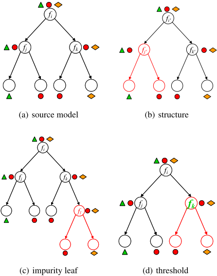
Random forest. Random forest aims to learn a classifier R consisting of M decision trees {h1, h2, . . . , hM} when dataset DS = {(xS1 , yS 1 ) , (xS2 , yS 2 ) , . . . , (xSnS , yS nS )} is given. The output of hj on sample xSi is (h1j (xSi ), h2j (xSi ), . . . , hLj (xSi )), where hlj (xSi ) is the output of hj on the Yl class. To build the jth individual tree, random forest uses the bootstrap sampling strategy to select a subset DS j , containing nS instances, from DS . For each split of the jth tree, feature randomization is used to select k features from the feature space K, and then the optimal feature is chosen from the candidate feature set according to splitting criteria. The output of R is computed by majority voting: H (xSi ) = Yargmax l ∑Mi=1 wjhlj (xSi ).
4 Method
FAT is a model transfer method that transfers the given source model to the target domain, relying on a relatively small labeled training set. It can adapt an existing cognitive assessment model to new evaluation tasks. In [Utgoff, 1989], the influence factors that hinder the rebuilding of tree models are summarized as a non-linear function:
where K is the number of features (i.e., |xSi | or |xTi |), P is the maximum number of possible values of a feature, and N is the number of instances (i.e., nT ). The cost of model adaptation is indeed proportional to the size of the sample space, and the size and diversity of feature space when the source models are transferred to the target. Specifically:
- The selection of splitting feature influences the structure of individual trees. When the number of distinguished features K increases or the feature set changes, the optimal structures of decision trees transform [Figure 1(b)].
- Suboptimal combination of splitting features causes the impurity of leaf nodes, which can expand to a full subtree [Figure 1(c)].
- Same problem shares similar tree structure. However, with the change of possible values of features P, there is still some thresholds that need to be adjusted [Figure 1(d)].
4.1 IGME
Most model transfer learning algorithms assume that individual learners for similar tasks share some structures or parameters [Pan and Yang, 2010]. According to the evaluation criterion of the individual decision trees [Utgoff, 1989], there are multi-level of similarities or model inadaptability, i.e., wrong structure, impurity of leaf nodes and threshold inadaptability. One of the popular ensemble model adaptation mechanisms is by personalizing the growth strategy for each individual classifier [Hu et al., 2018]. The proposed IGME method belongs to this category. The basic idea of IGME is to evaluate individual learners according to the information gain of split features. We rank every individual tree, and update its structure or parameter personalized. In the process of model rebuilding, the most crucial challenge is to quantify the level of inadaptability. In this section, we propose a new scoring rule, i.e., information gain based model evaluation (IGME) strategy. It jointly reflects both the accuracy and splitting feature distribution of individual classifiers.
In information theory, the information gain is used to measure the quality of a split:
where, a is the split feature. Ent(D) = - ∑Lk=1 pk log2 pk is the information entropy of the dataset D and pk is the proportion of the kth category of samples in dataset D. Ent(D|a) = ∑Vv=1 |Dv | |D| Ent(Dv ) is the conditional entropy when using feature a to split D into V partitions. Information gains of all features form an information gain set IG(D, X). To measure the value of information gain, we sort IG(D, X), and we use IGR(D,X) to represent the sequence number of every feature. For example, if IG(D,X) is {2.3, 6.7, 4.5, 1.2}, then IGR(D, X ) is {3, 1, 2, 4}.
Assume Aj is the features set to build the jth individual tree, IG(DS ,Aj) is the information gain set for the source domain and IG(DT ,Aj) is for the target domain. IGR(DS ,Aj) and IGR(DT ,Aj) are the sequence set. The following metric is defined to measure each individual tree:
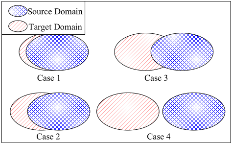
where ∣∣IGR(DS , a) - IGR(DT , a)∣∣ measures the importance difference for feature a. Plus one +1 is to prevent the occurrence of IGR(DS , a) = IGR(DT , a). S(hj) defines four degrees of coupling (Figure 2):
- Case 1: the value of S(hj) is very small. Almost all features that used to construct the jth tree have equal importance in the target domain.
- Case 2: the value of S(hj) increases slightly. Most of the features to construct the jth tree have equal importance in the target domain.
- Case 3: only a few features that used to construct the ith tree have equal importance in the target domain.
- Case 4: the value of S(hj) is very big. Almost no features that used to construct the jth tree is important in the target domain.
Also, testing accuracy of the target domain is also significant in evaluating an individual tree. So, we combine initial S(hi) and testing accuracy of the target domain, and redefine this metric:
where sgn(x) is sign function and λ is the weight coefficient. In the first part of Equation 4, IGME regularizes the value of feature coupling with |Aj| to make sure the range of this part in [0, 1/2]. In the last part of Equation 4, the error rate of hj is also limited to [0, 1/2].
4.2 DATG
According to Equation 4, there are four degrees of adaptability for individual tree. We need to update the existing model according to S(hj). Thus, we define three domain adaptation tree growing (DATG) mechanism for individual tree.
Modify the Subtree
The core issue in Modify The Subtree (MTS) is to determine the subtrees that should be modified. Assume node v divides
Algorithm 1 Modify The Subtree (MTS)
Input: Subtree v, labeled samples in target domain S, max
depth of decision tree dm, current depth dc Output: Subtree v 1: function MTS(v, S, dm, dc) 2: if |S| == 0 then % no instance arrives 3: set v as leaf node; return v 4: end if 5: if v is leaf node then % leaf node 6: return v 7: end if 8: P = v.substlft; Q = v.substrgt 9: calculate DI according to Equation 5 10: if DI < thres then 11: v = buildT ree(S) 12: else 13: v.childl = MT S(v.childl, P, dm, dc + 1) 14: v.childr = MT S(v.childr, Q, dm, dc + 1) 15: end if 16: return v 17: end functiondataset S into two parts, the left subset P = v.substlft and the right subset Q = v.substrgt. To evaluate the splitting ability of the internal nodes, we define distribution divergence to measure the distribution of the left and the right subset:
where dm is the maximum depth of decision tree, dc is current depth of node v, and M = (P +Q)/2. Y is label space of the target domain. Distribution divergence relies on JensenShannon divergence and Kullback-Leibler divergence (Equation 6). We weight the distribution divergence with logdm (dc) to make sure the shallow nodes have a bigger modification chance. MTS defines a top-bottom working procedure, and the pseudo-code of MTS is shown in Algorithm 1.
Split Leaf Nodes
Split Leaf Nodes (SLN) is designed to deal with the impurity leaf nodes. In some cases, the existing splitting features in one tree are hard to split all instances in the target domain and we need to add new features to expand the existing models. The pseudo-code of SLN is presented in Algorithm 2. The leaf nodes v will be retrained if the arrived dataset S satisfies two conditions: 1) The size of S is greater than predefined threshold values; 2) Dataset S contains at least two categories of instances.
Update Feature Threshold
Update Feature Threshold (UFT) is inspired by the fact that decision trees exhibit structural similarity in similar problems [Segev et al., 2017]. For example, if we design a touchscreen based cognitive assessment task, and run this task on two devices with different sizes of touchscreen. Data acquired
Algorithm 2 Split Leaf Nodes (SLN)
Input: Subtree v, labeled samples in target domain S Output: Subtree v 1: function SLN(v, S) 2: if |S| == thres || categoryNum(S) > 1 then 3: return v 4: end if 5: if v.isLeaf then 6: v = buildT ree(S) 7: else 8: v.childl = SLN(v.childl, v.substlf t) 9: v.childr = SLN(v.childr, v.substrgt) 10: end if 11: return v 12: end functionAlgorithm 3 Update Feature Threshold (UFT) Input: Subtree v, labeled samples in target domain S Output: Subtree v 1: function UFT(v, S) 2: if |S| == 0 then 3: d(v) = 0 4: return v 5: end if 6: if d(v) == 0 then 7: y(v) ← arg max y |{(·, y) ∈ S}| 8: return v 9: end if 10: v ← upadateT hresholds(v, S) 11: if d(v) == 0 then 12: return v 13: end if 14: v.childlef t = UF T (v.childlef t, v.subsetlef t) 15: v.childright = UF T (v.childright, v.subsetright) 16: return v 17: end functionwith both devices share many features and dependencies (e.g., times and velocity). However, the scale of features differs between different devices. Thus, the thresholds of splitting features also differ between different domains. UFT updates the threshold of every splitting feature top-down, and the pseudocode of UFT is presented in Algorithm 3. For internal nodes with the non-empty arriving dataset, UFT recalculates the optimal threshold according to information gain.
4.3 Fine-Grained Adaptation RandomForest
Algorithm 4 presents the pseudo-code of FAT. Existing ensemble model for source domain R and the information gain of source domain IG(DS ,X) are used as the input of FAT. Firstly, FAT calculates information gain of the target domain and predicts the classification result of the existing model on DT . Then, all individual classifiers are measured by S(hj) metric. Finally, AFA adapts each decision tree with different strategies to realize fine-grained domain adaptation.
Algorithm 4 Fine-Grained Adaptation Random Forest (FAT)
Input: Ensemble classifier R, source domain DT , coefficient λ, information gain of source domain IG(DS ,X), max depth of decision tree dm, update threshold δ1 <
δ2 < δ3 Output: Classifier R 1: function FAT(R,DT ) 2: calculate IG(DT , X) for target domain 3: calculate IGR(DS , X ) and IGR(DT , X ) 4: for each individual tree hj ∈ R do 5: Aj = splitFeature(hj) % calculate feature set 6: for each instances (xTi , yT i ) ∈ DT do 7: hj(xTi ) = predict(hj, xTi ) 8: end for 9: calculate S(hj) according to Equation 4 10: if S(hj) < δ1 then 11: hj = buildTree(S T ); continue 12: end if 13: if S(hj) < δ2 then 14: hj = MTS(hj , ST , maxD, 1); continue 15: end if 16: if S(hj) < δ3 then 17: hj = SLN(hj , ST ); continue 18: end if 19: if S(hj) ≥ δ3 then 20: hj = UFT (hj , ST ); continue 21: end if 22: end for 23: return R 24: end function5 Experiments and Analysis
In this section, we evaluate the performance of FAT via extensive experiments on the cognitive assessment dataset.
5.1 Datasets and Preprocessing
Cognitive Assessment Tasks
We use a touchscreen based cognitive assessment test (based on the Box and Block test [Mathiowetz et al., 1985]) to evaluate the cognitive state of older adults, which includes four different kinds of single-tasks and 12 different kinds of dual-tasks. Four single-tasks are single-task I (move block from start area to target area one by one, Figure 3(a)), single-task II (move block from start area to specific target areas, Figure 3(b)), single-task III (move block from start area to target areas sequentially, Figure 3(c)), and single-task IV (move block from start area to fixed target area, Figure 3(d)). Twelve dual-tasks are combinations of four single-tasks and three language ability related tasks, i.e., speaking while doing single-task, including dual-task BI, CI, DI, BII, CII, DII, BIII, CIII, DIII, BIV, CIV, DIV. These three language ability related tasks are series 1s (A: counting backward from 100), animal names (B: enumerating animal names), series 7s (C: subtracting seven from 100).

| S | T | STL | TCA | GFK | Src | Tar | Com | Ser | Struct | Mix | FAT | |
|---|---|---|---|---|---|---|---|---|---|---|---|---|
| I | II | .533±.01• | .561±.00• | .613±.00• | .661±.01• | .624±.01• | .637±.01• | .689±.01• | .665±.01• | .735±.01• | .827±.00 | |
| I | AII | .492±.01• | .547±.01• | .504±.00• | .667±.01• | .557±.01• | .672±.01• | .738±.01• | .602±.01• | .697±.01• | .854±.00 | |
| I | BII | .407±.01• | .533±.00• | .680±.00• | .598±.01• | .615±.01• | .632±.01• | .603±.01• | .489±.01• | .613±.02• | .744±.00 | |
| I | CII | .561±.01• | .551±.00• | .601±.00• | .542±.00• | .567±.00• | .588±.01• | .616±.01• | .520±.01• | .620±.01• | .788±.00 | |
| II | II | .394±.00• | .492±.00• | .533±.00• | .670±.01• | .633±.00• | .687±.01• | .690±.01• | .631±.01• | .722±.01• | .838±.00 | |
| II | AII | .509±.00• | .460±.00• | .493±.00• | .677±.01• | .572±.01• | .644±.00• | .669±.00• | .581±.01• | .705±.00• | .832±.00 | |
| II | BII | .355±.01• | .449±.01• | .488±.00• | .591±.01• | .595±.01• | .603±.01• | .605±.01• | .531±.01• | .587±.01• | .792±.00 | |
| II | CII | .501±.00• | .536±.00• | .517±.00• | .585±.01• | .645±.01• | .651±.01• | .684±.01• | .585±.01• | .647±.01• | .803±.00 | |
| TL→VS | III | II | .489±.01• | .555±.00• | .646±.00• | .669±.01• | .557±.01• | .625±.01• | .669±.01• | .705±.01• | .672±.01• | .794±.00 .837±.00 |
| III | AII | .467±.01• | .574±.00• .488±.00• | .630±.00• .539±.00• | .661±.01• | .557±.01• .584±.01• | .639±.00• .615±.01• | .655±.01• .613±.01• | .610±.01• .559±.01• | .653±.01• .607±.01• | .811±.00 | |
| III III | BII CII | .445±.01• .463±.00• | .505±.00• | .520±.00• | .598±.01• .565±.01• | .540±.01• | .627±.01• | .612±.01• | .604±.01• | .616±.01• | .763±.00 | |
| IV | II | .452±.00• | .547±.00• | .490±.00• | .631±.00• | .581±.00• | .651±.00• | .619±.00• | .792±.01 | .602±.00• | .781±.00 | |
| IV | AII | .479±.01• | .578±.01• | .554±.00• | .661±.01• | .607±.01• | .661±.01• | .687±.01• | .639±.01• | .673±.01• | .805±.00 | |
| IV | BII | .291±.00• | .537±.01• | .611±.00• | .611±.01• | .640±.01• | .600±.02• | .617±.00• | .514±.01• | .669±.01• | .817±.00 | |
| IV | CII | .468±.01• | .535±.00• | .586±.00• | .566±.01• | .576±.01• | .617±.00• | .647±.01• | .609±.01• | .649±.01• | .787±.00 | |
| II | I | .555±.00• | .511±.00• | .551±.00• | .631±.00• | .595±.00• | .679±.00• | .669±.00• | .617±.00• | .611±.01• | .739±.00 | |
| II | II | .419±.00• | .430±.00• | .357±.00• | .690±.00• | .566±.01• | .654±.01• | .695±.00• | .666±.01• | .688±.01• | .849±.00 | |
| II | III | .534±.00• | .529±.00• | .515±.00• | .619±.01• | .520±.00• | .617±.01• | .648±.00• | .618±.00• | .614±.00• | .745±.00 | |
| .494±.01• | .520±.01• | .530±.00• | .699±.00• | .685±.01• | .725±.00• | .696±.01• | .776±.00 | |||||
| II AII | IV | .539±.00• | .516±.00• | .536±.00• | .623±.00• | .652±.01• | .609±.00• | .696±.00• | .698±.01• | .633±.01• | .763±.00 | |
| AII | I II | .443±.00• | .469±.00• | .546±.00• | .670±.00• | .544±.00• .609±.00• | .650±.00• | .700±.00• | .572±.00• .592±.01• | .732±.01• | .855±.00 | |
| VS→TL | AII | III | .492±.00• | .525±.00• | .458±.00• | .597±.01• | .575±.01• | .649±.01• | .650±.00• | .618±.00• | .630±.00• | .734±.00 |
| AII | IV | .542±.00• | .517±.00• | .601±.00• | .691±.00• | .654±.01• | .713±.00• | .750±.00• | .751±.01• | .702±.00• | .800±.00 | |
| BII | I | .508±.00• | .440±.00• | .441±.00• | .640±.01• | .513±.00• | .637±.00• | .693±.00• | .582±.01• | .636±.00• | .783±.00 | |
| BII | II | .468±.01• | .353±.01• | .323±.00• | .654±.01• | .540±.00• | .664±.00• .655±.00• | .704±.00• | .671±.01• | .690±.01• | .843±.00 | |
| BII | III IV | .529±.01• .469±.01• | .550±.01• .485±.00• | .429±.00• .526±.00• | .580±.00• .654±.01• | .593±.00• .619±.00• | .690±.00• | .662±.00• .706±.01• | .623±.00• | .658±.01• .723±.01• | .744±.00 .786±.00 | |
| BII | I | .509±.01• | .484±.00• | .594±.00• | .623±.01• | .550±.00• | .652±.00• | .661±.00• | .719±.01• | .637±.01• | .771±.00 | |
| CII | II | .521±.01• | .491±.01• | .579±.00• | .682±.01• | .575±.01• | .667±.01• | .682±.00• | .612±.01• .689±.00• | .716±.00• | .864±.00 | |
| CII | III | .481±.01• | .529±.01• | .637±.00• | .613±.01• | .689±.00• | .650±.00• | .626±.01• | .661±.00• | .747±.00 | ||
| CII | IV | .548±.01• | .586±.00• | .724±.00• | .581±.00• | .693±.00• | .697±.01• | .793±.00 | ||||
| CII | AII | .634±.01• | .542±.01• | .686±.00• | .672±.01• | .655±.00• | .689±.01• .820±.00• | .740±.00• | .673±.00• | .677±.00• | .928±.00 | |
| II | BII | .581±.01• | .600±.01• | .539±.00• .539±.00• | .586±.01• | .783±.00• .707±.01• | .782±.00• | .689±.00• | .571±.02• | .699±.00• .674±.01• | .846±.00 | |
| II | CII | .527±.00• | .466±.01• | .493±.00• | .604±.01• | .615±.00• | .737±.01• | .694±.01• | .632±.01• | .706±.01• | .884±.00 | |
| II AII | II | .615±.01• | .668±.01• | .741±.00• | .670±.01• | .797±.00• | .817±.00• | .787±.01• | .718±.01• | .785±.01• | .913±.00 | |
| AII | BII | .559±.01• | .573±.01• | .657±.00• | .655±.01• | .638±.00• | .753±.00• | .670±.00• | .668±.01• | .665±.01• | .863±.00 | |
| VS→VS | AII | CII | .484±.01• | .534±.01• | .431±.00• | .623±.01• | .612±.00• | .750±.01• | .664±.01• | .666±.01• | .635±.01• | .875±.00 |
| BII | II | .481±.02• | .550±.01• | .707±.00• | .667±.01• | .655±.00• | .672±.00• | .681±.00• | .724±.02• | .712±.01• | .854±.00 | |
| BII | AII | .532±.01• | .530±.00• | .516±.00• | .628±.01• | .617±.00• | .650±.00• | .653±.01• | .722±.01• | .675±.01• | .812±.00 | |
| BII | CII | .574±.00• | .558±.00• | .614±.00• | .613±.00• | .703±.00• | .768±.00• | .726±.00• | .806±.00• | .741±.00• | .885±.00 | |
| CII | II | .494±.02• | .515±.01• | .495±.00• | .617±.01• | .611±.00• | .628±.00• | .661±.01• | .688±.01• | .739±.01• | .797±.00 | |
| CII | AII | .510±.00• | .525±.00• | .660±.00• | .736±.00 | .678±.00• | .625±.00• | .657±.00• .687±.00• | .685±.00• .644±.00• | .682±.00• | .746±.00 | |
| CII | BII II | .565±.00• .550±.00• | .544±.00• .579±.00• | .592±.00• .577±.00• | .598±.00• | .648±.00• .584±.00• | .711±.00• .678±.00• | .669±.00• | .773±.00• | .825±.00 | ||
| I | III | .531±.00• | .565±.00• | .533±.00• | .660±.01• .627±.01• | .560±.00• | .674±.00• | .669±.00• | .688±.01• | .680±.01• | .839±.00 | |
| I | .615±.01• | .646±.00• | .762±.00 | |||||||||
| I II | IV I | .477±.00• | .556±.00• .548±.00• | .541±.00• .567±.00• | .650±.01• | .591±.01• | .695±.00• | .707±.00• .712±.00• | .653±.01• .629±.00• | .663±.00• .670±.01• | .798±.00 | |
| II | II | .490±.00• .464±.00• | .528±.00• | .597±.00• | .618±.01• .657±.01• | .514±.00• .578±.00• | .619±.00• .677±.00• | .696±.00• | .606±.00• | .652±.01• | .823±.00 .771±.00 | |
| II | IV | .453±.01• | .507±.00• | .619±.00• | .672±.01• | .581±.01• | .714±.00• | .697±.00• | .676±.01• | .711±.00• | .810±.00 | |
| TL→TL | III | I | .551±.01• | .597±.00• | .610±.00• | .613±.01• | .551±.00• | .659±.00• | .693±.00• | .624±.00• | .681±.00• | .801±.00 |
| III | II | .492±.01• | .535±.00• | .622±.00• | .679±.00• | .568±.00• | .681±.00• | .702±.00• | .696±.01• | .689±.00• | .856±.00 | |
| III | IV | .473±.00• | .621±.00• | .707±.00• | .737±.00• | .642±.01• | .700±.00• | .701±.01• | .684±.01• | .689±.01• | .836±.00 | |
| IV | I | .389±.00• | .588±.00• | .465±.00• | .663±.01• | .565±.00• | .651±.00• | .694±.01• | .669±.00• | .668±.00• | .811±.00 | |
| IV | II | .466±.00• | .608±.00• | .628±.00• | .667±.01• | .564±.00• | .711±.00• | .673±.00• | .624±.01• | .656±.01• | .814±.00 | |
| IV | III | .493±.00• | .587±.00• | .697±.00• | .637±.01• | .629±.00• | .721±.00• | .668±.00• | .617±.00• | .632±.00• | .777±.00 |
Data Collection
The prototype cognitive assessment tasks are implemented with the Android Studio platform 2.2.2. We collect data in two scenarios.
- In the first scenario (denoted by TL), the prototype system is run on Huawei M5 tablet with 10.1 inches, 1920 × 1200 pixels touchscreen. 61 subjects, including 20 subjects with mild cognitive decline (age: 68.25±6.15, eight males and 12 females) and 41 healthy controls (age: 67.36 ± 4.76, 21 males and 20 females), are recruited to participate in data collection. All subjects perform four single tasks (single-task I, II, III, IV).
- In the second scenario (denoted by VS), the prototype system is run on the NanoPi M4 board with 21.5 inches, 1920 × 1200 pixels touchscreen. 37 subjects, including 25 subjects with mild cognitive decline (age: 65.08 ± 9.68, 16 males and nine females) and 12 healthy controls (age: 39.44 ± 2.31, seven males and five females), are recruited to participate in data collection. All subjects perform one single-task (single-task II) and three dualtasks (dual-task AII, BII, CII).
Feature Extraction
Five categories of features are extracted from raw data, including number-based features (∈ R10 ), time-based features (∈ R50 ), velocity-based features (∈ R130 ), angle-based features (∈ R60 ), drop point distribution-based features (∈ R70 ).
5.2 ComparisonMethods and Parameters Details
We use SrcOnly (Src), TarOnly (Tar), ComOnly (Com) as the first three benchmarks. They are three trivial approaches that do not involve transfer learning, where we create comparative models with source data, part of target data, and the mixture of source data and part of target data respectively. Besides, FAT is compared with six state-of-the-art transfer learning methods, i.e., Structure Expansion/Reduction (SER), Structure Transfer (Struct), mix of SER and Struct (Mix) [Segev et al., 2017], Stratified Transfer Learning (STL) [Wang et al., 2018], Transfer Component Analysis (TCA) [Pan et al., 2011], and Geodesic Flow Kernel (GFK) [Gong et al., 2012]. Where, SER, Struct and Mix are model transfer methods based on random forest. TCA, STL and GFK are representative feature transfer methods, which transfer both source domain and target domain into unified feature space to reduce their distribution differences.
We conduct experiments on Lenovo ThinkStation desktop computer (Intel Core i7-6700/16GB DDR3) with Matlab R2018b platform. All nine comparison methods and FAT use random forest as the basic classifier. We set the number of trees in random forest M = 30. The number of candidate features for each node is set as √K, K is the total number of features. The minimum instance size for splitting a node is set as 2. The maximum depth for individual tress is set as maxD = 10. In addition, three transfer methods for feature knowledge (i.e., STL, TCA and GFK) require dimension reduction. Therefore, we set the dimension of feature as 30. δ1, δ2, δ3 in FAT are set to 0.6, 0.7, and 0.8 respectively.
5.3 Experimental Result
To compare FAT with other comparing methods, we use data collected in the first and the second scenario interchangeably as the source domain and the target domain. In each experiment, 30% of data in the target domain are used to finetune the existing source domain model, and the other 70% are used as the testing data. Since two scenarios each contain four tasks, there are a total of 56 combinations. Table 1 shows the diagnosis accuracy of FAT and nine other methods. The paired t-test at the significance level of 0.05 is used to measure whether FAT is statically superior to the comparing methods, where statical superiority is indicated with · and the best performance is marked with boldface. Some conclusions can be drawn from Table 1:
- FAT reaches competitive results with a maximum accuracy of 92.8% and a minimum accuracy of 73.4%, proving the effectiveness of the proposed method;
- FAT ranks 1st among all ten methods on 55/56 transfer tasks. When transferring from TL single-task IV to VS single-task II, the accuracy of FAT is inferior to the accuracy of Struct;
- FAT is significantly superior to all other comparing methods on 54/56 transfer tasks at the confidence level of 0.05. FAT does not achieve statically superior results only on two transfer tasks.
6 Conclusion
Cognitive health plays an important role for the well-being of older adults. However, limited by the mildness of early signs of cognitive decline and the small-sampling problem in detection model building, it is not easy to realize high accuracy diagnosis of cognitive impairment. In this paper, we propose a fine-grained domain adaptation method, namely FAT, to bridge the cross-tasks gap for cognitive assessment. FAT is a random forest based model transfer method, which transfers each individual classifier with different strategy to realize high-accuracy adaptation. The advantages of FAT are three-fold: 1) FAT updates the existing model with a small amount of samples in the target domain, alleviating the smallsampling challenge; 2) FAT is a random forest based transfer learning method, satisfied the interpretability need of diagnosis model; 3) FAT transfers each individual classifier with different strategy, which can realize high-accuracy model adaptation. Also, to evaluate the accuracy of FAT, we design 16 different cognitive assessment tasks and recruit healthy and MCI subjects to participate the evaluation experiments.
Acknowledgments
This work is supported by Key-Area Research and Development Program of Guangdong Province (No.2019B010109001), by the National Key Research and Development Plan of China (No.2017YFB1002801), by the Natural Science Foundation of China under Grant (No.61972383), and by Alibaba Group through Alibaba Innovative Research (AIR) Program.
@inproceedings{ijcai2020p597,
  title     = {Bridging Cross-Tasks Gap for Cognitive Assessment via Fine-Grained Domain Adaptation},
  author    = {Zhang, Yingwei and Chen, Yiqiang and Yu, Hanchao and Lv, Zeping and Li, Qing and Yang, Xiaodong},
  booktitle = {Proceedings of the Twenty-Ninth International Joint Conference on
               Artificial Intelligence, {IJCAI-20}},
  publisher = {International Joint Conferences on Artificial Intelligence Organization},
  editor    = {Christian Bessiere},
  pages     = {4330--4337},
  year      = {2020},
  month     = {7},
  note      = {Special track on AI for CompSust and Human well-being},
  doi       = {10.24963/ijcai.2020/597},
  url       = {https://doi.org/10.24963/ijcai.2020/597},
}
TY - CPAPER TI - Bridging Cross-Tasks Gap for Cognitive Assessment via Fine-Grained Domain Adaptation AU - Zhang, Yingwei AU - Chen, Yiqiang AU - Yu, Hanchao AU - Lv, Zeping AU - Li, Qing AU - Yang, Xiaodong T2 - Proceedings of the Twenty-Ninth International Joint Conference on Artificial Intelligence, IJCAI-20 PB - International Joint Conferences on Artificial Intelligence Organization PY - 2020 SP - 4330 EP - 4337 DO - 10.24963/ijcai.2020/597 UR - https://doi.org/10.24963/ijcai.2020/597 ER -Copied
Machine-readable versions of this paper, for tools and AI agents:





