
State Variable Effects in Graphical Event Models
Proceedings of the Twenty-Ninth International Joint Conference on Artificial Intelligence. Main track. Pages 4291-4297.
https://doi.org/10.24963/ijcai.2020/592
Keywords
- Uncertainty in AI: Uncertainty Representations
- Machine Learning: Learning Graphical Models
- Data Mining: Mining Spatial, Temporal Data
- Uncertainty in AI: Graphical Models
Abstract
Many real-world domains involve co-evolving relationships between events, such as meals and exercise, and time-varying random variables, such as a patient's blood glucose levels. In this paper, we propose a general framework for modeling joint temporal dynamics involving continuous time transitions of discrete state variables and irregular arrivals of events over the timeline. We show how conditional Markov processes (as represented by continuous time Bayesian networks) and multivariate point processes (as represented by graphical event models) are among various processes that are covered by the framework. We introduce and compare two simple and interpretable yet practical joint models within the framework with relevant baselines on simulated and real-world datasets, using a graph search algorithm for learning. The experiments highlight the importance of jointly modeling event arrivals and state variable transitions to better fit joint temporal datasets, and the framework opens up possibilities for models involving even more complex dynamics whenever suitable.
- [Bhattacharjya et al., 2018] D. Bhattacharjya, D. Subrama- nian, and T. Gao. Proximal graphical event models. In Adv. Neur. Inf. Process. Syst. (NeurIPS), pages 8147-8156, 2018.
- [Bhattacharjya et al., 2019] D. Bhattacharjya, K. Shan- mugam, T. Gao, N. Mattei, and K. R. Varshney. Event- driven continuous time Bayesian networks: An application in modeling progression out of poverty through integrated social services. In IJCAI Workshop on AI for Social Good (AI4SG), 2019.
- [Bhattacharjya et al., 2020] D. Bhattacharjya, K. Shan- mugam, T. Gao, N. Mattei, K. R. Varshney, and D. Subra- manian. Event-driven continuous time Bayesian networks. In Proc. of Conf. on Artif. Intell. (AAAI), 2020.
- [Cox and Lewis, 1972] D. R. Cox and P. A. W. Lewis. Mul- tivariate point processes. In Proc. of the Sixth Berkeley Symposium on Math. Stat. and Prob., Vol. 3: Probability Theory, pages 401-448, 1972.
- [Dean and Kanazawa, 1989] T. Dean and K. Kanazawa. A model for reasoning about persistence and causation. Computational Intelligence, 5:142-150, 1989.
- [Didelez, 2008] V. Didelez. Graphical models for marked point processes based on local independence. J. R. Stat. Soc. B, 70(1):245-264, 2008.
- [Downs and Vogel, 1993] J. J. Downs and E. F. Vogel. A plant-wide industrial process control problem. Computers & Chemical Engineering, 17(3):245-255, 1993.
- [Du et al., 2016] N. Du, H. Dai, R. Trivedi, U. Upadhyay, M. Gomez-Rodriguez, and L. Song. Recurrent marked temporal point processes: Embedding event history to vec- tor. In Proc. SIGKDD Int. Conf. Knowledge Discovery and Data Mining (KDD), pages 1555-1564, 2016.
- [Eichler, 1999] M. Eichler. Graphical Models in Time Series Analysis. PhD thesis, University of Heidelberg, Germany, 1999.
- [Frank and Asuncion, 2010] A. Frank and A. Asuncion. UCI machine learning repository, 2010.
- [Gao et al., 2020] T. Gao, D. Subramanian, K. Shanmugam, D. Bhattacharjya, and N. Mattei. A multi-channel neural graphical event model with negative evidence. In Proc. of Conf. on Artif. Intell. (AAAI), 2020.
- [Goulding et al., 2016] J. Goulding, S. Preston, and G. Smith. Event series prediction via non-homogeneous Poisson process modelling. In Proc. of IEEE Int. Conf. on Data Mining (ICDM), pages 161-170, 2016.
- [Gunawardana and Meek, 2016] A. Gunawardana and C. Meek. Universal models of multivariate temporal point processes. In Proc. of Int. Conf. on Artif. Intell. Stat. (AISTATS), pages 556-563, 2016.
- [Gunawardana et al., 2011] A. Gunawardana, C. Meek, and P. Xu. A model for temporal dependencies in event streams. In Adv. Neur. Inf. Process. Syst. (NeurIPS), pages 1962-1970, 2011.
- [Kolar et al., 2010] M. Kolar, L. Song, A. Ahmed, and E. P. Xing. Estimating time-varying networks. The Annals of Applied Statistics, 4(1):94-123, 2010.
- [Kumar et al., 2016] S. Kumar, F. Spezzano, V. S. Subrah- manian, and C. Faloutsos. Edge weight prediction in weighted signed networks. In Proc. of Int. Conf. on Data Mining (ICDM), pages 221-230. IEEE, 2016.
- [Leskovec and Krevl, 2014] J. Leskovec and A. Krevl. SNAP Datasets: Stanford large network dataset collection. http://snap.stanford.edu/data, June 2014. Link
- [Meek, 2014] C. Meek. Toward learning graphical and causal process models. In Proc. of UAI Workshop on Causal Inference: Learning and Prediction, pages 43-48, 2014.
- [Murphy, 2002] K. Murphy. Dynamic Bayesian Networks: Representation, Inference and Learning. PhD thesis, Uni- versity of California Berkeley, USA, 2002.
- [Nodelman et al., 2002] U. Nodelman, C. R. Shelton, and D. Koller. Continuous time Bayesian networks. In Proc. of Conf. on Uncertainty Artif. Intell. (UAI), pages 378-378, 2002.
- [Nodelman et al., 2003] U. Nodelman, C. R. Shelton, and D. Koller. Learning continuous time Bayesian networks. In Proc. of Conf. on Uncertainty Artif. Intell. (UAI), pages 451-458, 2003.
- [Parikh et al., 2012] A. P. Parikh, A. Gunawardana, and C. Meek. Conjoint modeling of temporal dependencies in event streams. In Proc. of UAI Workshop on Bayesian Modeling Applications, August 2012.
- [Pearl, 2014] J. Pearl. Probabilistic Reasoning in Intelligent Systems: Networks of Plausible Inference. Morgan Kauf- mann, 2014.
- [Plis et al., 2015] S. Plis, D. Danks, C. Freeman, and V. Cal- houn. Rate-agnostic (causal) structure learning. In Adv. Neur. Inf. Process. Syst. (NeurIPS), pages 3303-3311, 2015.
- [Rajaram et al., 2005] S. Rajaram, T. Graepel, and R. Her- brich. Poisson-networks: A model for structured point processes. In Proc. Int. Workshop Artif. Intell. Stat. (AIS- TATS), pages 277-284, 2005.
- [Simma and Jordan, 2010] A. Simma and M. I. Jordan. Modeling events with cascades of Poisson processes. In Proc. of Conf. on Uncertainty Artif. Intell. (UAI), pages 546-555, 2010.
- [Weiss and Page, 2013] J. C. Weiss and D. Page. Forest- based point process for event prediction from electronic health records. In Machine Learning and Knowledge Dis- covery in Databases, pages 547-562, 2013.
- [Xiao et al., 2017] S. Xiao, J. Yan, X. Yang, H. Zha, and S. M. Chu. Modeling the intensity function of point pro- cess via recurrent neural networks. In Proc. of Conf. on Artif. Intell. (AAAI), pages 1597-1603, 2017.
- [Zhou et al., 2010] S. Zhou, J. Lafferty, and L. Wasserman. Time varying undirected graphs. Machine Learning, 80(2- 3):295-319, 2010.
References were extracted automatically from the PDF and may contain errors.
Full text extracted automatically from the PDF; figures, tables and equations may differ. The PDF is the version of record.
1 Introduction &RelatedWork
Several domains involve an underlying causal mechanism with co-evolving dynamics where the states of uncertain variables and their transitions influence arrivals of events, and vice versa. We make a semantic distinction between two kinds of variables - event labels and state (or system) variables. Event labels are categories of events, occurring instantaneously and often irregularly on the timeline. In contrast, state variables are variables which always exist in some state, with potential state changes observed at irregularly timed transitions. For instance, meals and exercise could be viewed as event labels, whereas a patient's blood glucose level (say with states for low, medium and high) is a state variable.
There is substantial literature on graphical models for dynamic systems. A useful distinction between the various avenues of research is based on whether observations are in discrete or continuous time. Dynamic Bayesian networks [Dean and Kanazawa, 1989; Murphy, 2002] are discrete-time models that extend Bayesian networks [Pearl, 2014] by jointly representing a set of discrete variables at regular epochs. Time series data are continuous valued measurements, typically also observed at regular epochs, and can be represented by Granger causal graphs [Eichler, 1999]. A stream of graphical modeling work for time series however also attempts to handle irregular observations such as through using additional labels for missing data [Kolar et al., 2010; Zhou et al., 2010] or through a sampling-rate-agnostic learning approach [Plis et al., 2015].
There is a vast body of burgeoning research on temporal processes for modeling multivariate streams of events, spanning parametric approaches and neural network architectures [Rajaram et al., 2005; Simma and Jordan, 2010; Weiss and Page, 2013; Goulding et al., 2016; Du et al., 2016; Xiao et al., 2017; Gao et al., 2020]. Such models use a marked point process [Cox and Lewis, 1972] to capture the continuous-time dynamics in event streams, varying in assumptions and parametrization around the historical dependencies between the various types of events. Graphical event models (GEM) [Didelez, 2008; Meek, 2014] are a highlevel framework for representing marked point processes in a graphical form; the framework subsumes a large class of temporal models for events.
Continuous time Bayesian networks (CTBN) [Nodelman et al., 2002] are a related model that represent conditional Markov processes where a joint set of variables make state transitions in an inter-dependent fashion. Some recent work on event-driven CTBNs (ECTBN) provides an extension enabling the effect of external events on state variables [Bhattacharjya et al., 2019; Bhattacharjya et al., 2020]. However, this model is limited in handling joint dynamics - it retains Markovian dependence between state variables and does not permit them to affect event arrivals, as can be common in numerous applications.
Our main contribution in this paper is a novel unifying framework that we refer to as a state variable graphical event model (SVGEM); this family of models jointly captures the co-evolution of state variables and event label arrivals in continuous time. The framework extends beyond the Markov assumptions in CTBNs/ECTBNs, and allows for state variables and event labels to dynamically influence each other, potentially in complex ways. It is therefore capable of representing a wide variety of process models. We theoretically demonstrate the generality of the SVGEM framework, showing how it encapsulates many models and existing frameworks including GEMs. Through experiments on simulated and realworld benchmark datasets, two specific models from the proposed framework are shown to outperform various baselines, highlighting the promising modeling power of the high-level framework.
2 Model Formulation
2.1 Basic Notation &Terminology
Variables & Data. We distinguish between two kinds of variables. Event labels are denoted E = {Ej}Jj=1 . We assume there is data about events occurring over time, DE = (tk, ek)NE k=1 , where tk are ordered time stamps between initial time t0 = 0 to the end time T , and ek belong to the event label set E. Discrete state variables are denoted X = {Xi}Ii=1 . Let Val(Xi) be the domain of variable Xi and Val(X) the domain of the set of state variables X. Data about each variable is of the form of state transitions, DXi = (tk, xk)Ni k=0 up to end time T, where the state at time t0 is the initial state and xk+1 ̸= xk ∀k, xk ∈ Val(Xi). Data for all state variables taken together is denoted DX = ⋃X∈X DX.
Definition 1. An occurrence refers to either an event label arrival or a state variable transition, i.e. an occurrence is of the form (tk, zk) where zk is either an event label, ek ∈ E, or a state of a state variable, xk ∈ Val(X),X ∈ X. Here zk is the occurrence label.
We use DZ to denote data of all occurrences pertaining to both kinds of variables in Z, and D = DE,X to denote data for all occurrences of all model variables.
Historical Dependence. The dynamics of event label arrivals and state variable transitions are driven by historical dependencies. We use h(·) to denote historical occurrences of either type of variable, i.e. event arrivals or state variable transitions. Consider variables Z = {ZE ,ZX }, where ZE and ZX are sets of event labels and state variables respectively. Then hZE (t) = {(tk, ek) ∈ DZE : tk < t} represents the history of event arrivals in the set ZE ⊂ E until time t, and hZX (t) = {(tk, xk) ∈ DZX : tk < t} represents the history of state variable transitions associated with the set ZX ⊂ X until time t. The combined history is hZ(t) = hZE (t) ∪ hZX (t). h∗Z(t) refers to the most recent occurrence label in the history hZ(t).
2.2 The SVGEMFramework
We now have the notation and terminology required to formalize the general SVGEM framework:
Definition 2. An SVGEMMincludes:
- A directed (possibly cyclic) graph G where:
- Every event label E ∈ E has parents UE = {UEE ,UXE }, where UEE ⊆ E and UXE ⊆ X are event label and state variable parents respectively
- Every state variable X ∈ X has parents UX = {UEX ,UXX }, where UEX ⊆ E and UXX ⊆ {X \ X} are event label and state variable parents respectively
- An initial distribution P0X over state variables
- Conditional intensity rate parameters Λ as follows:
- Every event label E ∈ E occurs with rate λE|hUE (t) at time t, where hUE (t) denotes the history of all occurrences in parent set UE; each set is denoted ΛE
- Every transition s, s′ for every state variable X ∈ X, s, s′ ∈ Val(X); s ̸= s′ , occurs with rate λs,s′ X|hUX (t) at time t when h∗X (t) = s, and 0 otherwise, where hUX (t) denotes the history of all occurrences in parent set UX; each set is denoted ΛX
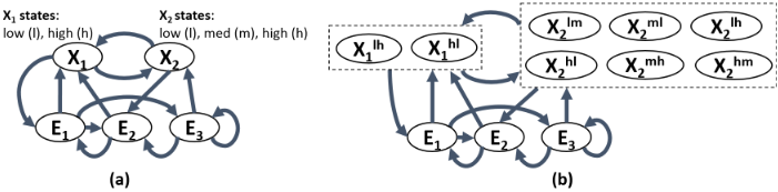
An SVGEM captures the joint dynamics of all occurrences based on an underlying graph that specifies the causal factors influencing each variable. Fig. 1(a) shows an illustrative SVGEM graph involving 2 state variables and 3 event labels. We highlight that the definition imposes an important constraint: a state variable cannot transition from state s to s′ if it is not already in state s. Also, note that an SVGEM is merely a framework or a family of models, similar to a GEM - for a fully specified generative model, more details about the general historical dependence (denoted by ΛE and ΛX) need to be provided, such as what is described next.
2.3 Types of Historical Dependence
We categorize various kinds of historical dependence for either type of variable. These are by no means exhaustive but cover the cases required for this article. All of these are stationary in the sense that an occurrence's rate is independent of the time at which history is considered, given the history.
- A historical dependence is Markov w.r.t set Z if the rate at any time t depends only on h∗Z(t), i.e. the most recent occurrence label in the history hZ(t).
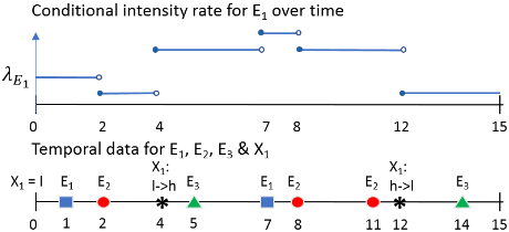
- A historical dependence is piece-wise constant (PC) w.r.t set Z if there is a fully specified mapping from the history hZ(t) at any time t into some discrete state space Σ [Gunawardana et al., 2011]. Such a mapping induces the conditional intensity rate for a variable to be piece-wise constant over the timeline for any dataset. Fig. 2 (Top) illustrates this by displaying the conditional intensity rate profile for an event label on an example dataset.
- A historical dependence is proximal w.r.t event label set ZE if the rate at any time t depends only on whether or not each node in ZE has occurred in a preceding time window before t [Bhattacharjya et al., 2018]. Proximality w.r.t state variables ZX needs further clarification, and is deferred to later in the article. We note that this is a special but important case of PC historical dependence.
- A historical dependence is restricted by a subset W of set Z if the rate at any time t is 0 when the most recent occurrence label h∗Z(t) belongs to W. Thus, if the most recent occurrence is fromW, the occurrence under consideration is impossible.
2.4 Equivalent GEM for an SVGEM
We define an expanded GEM, where each state variable transition is treated as an event, that can represent the dynamic process for an underlying SVGEM. Recall that nodes E ∈ E
and X ∈ X in the original SVGEM have parents UE = {UEE ,UXE } and UX = {UEX ,UXX } respectively. The expanded GEM that is constructed only includes event labels, and the parents for a node E in this GEM are denoted U′E .
Definition 3. The equivalent GEM for an SVGEM includes:
- A directed (possibly cyclic) graph with:
- A node Ei for every event label Ei ∈ E and a node Es,s′ j for every possible state transition s, s′ of every state variable Xj ∈ X in the SVGEM
- Directed arcs as follows: (i) for all Ei, retain arcs in UEEi and add arcs emanating from all Es,s′ j corresponding to Xj ∈ UXEi ; (ii) for all Es,s′ j corresponding to Xj, add arcs from all UEXj , all Es,s′ k corresponding to Xk ∈ UXXj , and all Es,s′ j corresponding to Xj (including the self loop).
- Conditional intensity rate parameters as follows:
- For all Ei, the intensity rate remains the same and is determined by historical arrivals of all parent event labels in the GEM, λEi|hU′Ei (t) = λEi|hUEi (t)
- For all Es,s′ j corresponding to Xj, historical dependence is restricted by the set of nodes {Es0 ,s′′ j } where s′′ ̸= s, otherwise it is equal to the corresponding rate in the SVGEM, λEs,s′ j |hU′Es,s′ j (t) = λs,s′ Xj |hUXj (t)
Theorem 4. The dynamic process represented by an SVGEM is identical to that of its equivalent GEM.
Proof. (Outline) The proof follows from the construction of the eqv. GEM. Event arrivals in both the SVGEM and the eqv. GEM follow the same process since the label set and corresponding intensity rates are identical. For state variables, there is a new set of event labels in the eqv. GEM, rates for which are restricted based on the constraint around state transitions. This ensures that transition events in the eqv. GEM process occur at the same rate as the SVGEM process only when it is feasible for the transition to happen.
An equivalent GEM for an SVGEM replaces state variables with an event label for every possible state variable transition. Def. 3 formalizes the graph construction and determination of the conditional intensity rates in the equivalent GEM. Fig. 1(b) shows the equivalent GEM for the SVGEM in (a). Since it is necessary to add several arcs to correctly capture the temporal dynamics, we avoid diagram clutter by keeping these arcs implicit using boxes over the new event labels.
We argue that an SVGEM is typically a better representation than its equivalent GEM for communicating with the user (or decision maker) because:
- An SVGEMmakes the semantic difference between the two types of variables self-evident.
- An SVGEM can be much more compact, particularly if there are several possible state variable transitions - with a reduction from ∑i (|Val(Xi)| ∗ |Val(Xi) - 1|) to |X | additional nodes in the graph - and therefore easier to interpret (see Fig. 1).
- Incorporating the constraint regarding state variables is trickier and more difficult to identify in the equivalent GEM as compared to the SVGEM (see Def. 3).
The notion of the equivalent GEM is still however a useful tool for computational reasons. For instance, this equivalence can be used to compute the log likelihood while learning specific parametric SVGEMs using temporal datasets.
2.5 Generality of SVGEMs
The following theorem formalizes the generality of the SVGEM framework by specifying some important model families in the literature.
Theorem 5. (i) A GEM [Didelez, 2008; Gunawardana and Meek, 2016] is an SVGEM without state variable nodes. (ii)
A CTBN [Nodelman et al., 2002] is an SVGEM without event label nodes and where state variables are Markov w.r.t their (state variable) parents. (iii) An ECTBN [Bhattacharjya et al., 2020] is an SVGEM with no arcs from state variables to event labels and where state variables are Markov w.r.t their state variable parents.
Proof. (Outline) An SVGEMwithout state variables only has nodes E with intensity rates λE|hUEE (t); this is howGEMs are defined. Removing event labels entirely instead and assuming Markov historical dependence results in a conditional Markov process. Incorporating the labels back but disabling arcs from state variables to events results in a set of conditional Markov processes that depend on historical event occurrences; thus the CTBN and ECTBN models are covered by the SVGEM framework as specified.
The following result makes a connection between Markov historical dependence in CTBNs (as well as ECTBNs) and piece-wise constant historical dependence.
Theorem 6. A CTBN and its extension ECTBN with proximal dependence w.r.t event label parents both involve PC historical dependencies for every node.
Proof. (Outline) In the specified ECTBN, state variables are Markov w.r.t their state variable parents and proximal w.r.t their event label parents. The transition rates therefore change from a constant to another when either the parent condition is modified due to a boundary window condition including an arrival of a parent label, or a transition of a state variable parent. A CTBN only has state variable parents and therefore only changes parameters at parent transitions. Event labels are proximal w.r.t each other in an ECTBN.
2.6 Two Specific SVGEMs
In the previous sub-section, we cast various models from the literature as special cases within the SVGEM framework. A case that is notably missing is where event labels are also affected by state variables, along with other event labels. This is common in numerous domains, for instance, a hospital is likely to be visited by patients with chronic conditions more often, and a manufacturing plant operating in varying modes exhibits different event trajectories.
We introduce two specific parametric models that simultaneously allow for influences in both directions. They are simple but practical models, and as we explain in the next section, easily learned from data. For model naming convention, assumptions about historical dependence for state variables are listed before event labels. Thus, the first 'MP' in 'MP MP' signifies that state variable nodes are Markov w.r.t their state variable parents and proximal w.r.t their event label parents, and the second 'MP' signifies the same for event label nodes.
SVGEM MP MP. In this SVGEM, a node is always Markov w.r.t its state variable parents and proximal w.r.t its event label parents. This is a natural generalization of ECTBN where in addition to state variable dynamics that depend on events in a proximal manner, an event's arrival rate depends on the current state of its state variable parents.
SVGEM MP PP. Here, state variable dynamics stay the same but now an event label node is proximal (not Markov) w.r.t its state variable parents. This is a unique view of dependence on state variables, where the historical occurrence time of a parent state variable transition within a recent window, as well as the nature of the transition, determine an event's arrival rate. In this fashion, historic state transitions are effectively treated as event labels, like in an equivalent GEM of an SVGEM. We consider the following 4 ways to categorize transitions into what are effectively new labels:
- all: all transitions are considered equivalent.
- each: each type of transition is a unique label.
- in: transitions going into a state are equivalent.
- out: transitions going out of a state are equivalent.
We show later through experiments that this particular nonMarkovian dependence of event arrivals on historical state transitions can often be a suitable fit for real-world data.
Theorem 7. SVGEM MP MP and SVGEM MP PP both involve PC historical dependencies for every node.
Proof. (Outline) State variables in both models have historical dependence similar to ECTBN, so the relevant part of Thm. 6 applies. In SVGEM MP MP, event labels are proximal w.r.t event label parents and Markov w.r.t state variable parents. Intensity rates therefore change from a constant to another when either the parent condition is modified due to a boundary window condition including a parent event arrival, or transition of a state variable parent. In SVGEM MP PP, event labels are proximal w.r.t an expanded label set and are piece-wise constant w.r.t the new change points.
Fig. 2 (Top) illustrates a piece-wise constant profile for the conditional intensity rate for label E1, modeled using SVGEM MP MP: it is Markov w.r.t X1 and proximal w.r.t E2. The figure indicates points on the timeline where the conditional intensity rate changes. Later we show that the above result is useful computationally during learning, since a piece-wise constant model simplifies the computation of parameters given the graph and other hyper-parameters.
3 Learning SVGEMs
G, P0X and Λ for an SVGEM can all be learned from data. Similar to models in the GEMs family, the parents for every node in an SVGEM can be learned separately and then combined to form the overall graph G. For the graph search procedure, we take a hill climbing score-based approach using the Bayesian information criterion (BIC) score, which is used to measure model fit performance in terms of the log likelihood of the model on a given dataset as well as the model complexity; since this approach is standard in the literature [Nodelman et al., 2003], here we focus primarily on the issue of learning parameters Λ given a graph.
If the parents of each node are known, then one can use the equivalent GEM notion of an SVGEM and ascertain that the log likelihood of a model with parameters Λ = {ΛX}, {ΛE} on an event dataset can be factorized as follows:
| Dataset | |X | | |E| | ∑i Ni | NE |
|---|---|---|---|---|
| Synthetic | 5 | 5 | ∼[35-45.8]K | ∼[15.1-16.9]K |
| Eastman | 16 | 18 | ∼[84-102.3]K | ∼[22.6-25.4]K |
| Diabetes | 1 | 11 | ∼6.2K | ∼14K |
| Bitcoin | 2 | 6 | 0 | ∼66.4K |
The computation of individual node log likelihoods is determined by the model parametrization, which depends on the assumptions about historical dependence. We summarize these below for our two proposed parametric SVGEMs. We use the following notation to represent an instantiation of parent sets: for a general node Z of either type, we introduce vector uZ = uXZ × uEZ , where uXZ is a joint instantiation of Z's state variable parents, i.e. from Val(UXZ ), and uEZ is a binary vector of indicators of Z's event label parents, each depending on whether it is present in some recent window.
SVGEM MP MP. The parameters in this model are Λ = {λE|uE ,QX|uX } ∀E,X, which includes intensity rates for event labels E for each parent instantiation uE and a set of conditional matrices for state variables X, one for each parent instantiation uX. From Thm. 7, this parametrization results in piece-wise constant historical dependence. One can therefore learn estimates for intensity rates through summary statistics on an event dataset [Gunawardana et al., 2011].
For example, for parent instantiation uE1 = {uX1 E1 = low, uE2 E1 = 0} of label E1, the maximum likelihood estimate computed on the event dataset in Figure 2 (Bottom) for ˆλE1|uE1 is 1/2. This is the rate at which E1 occurs given that X1 is in state 'low' and that E2 has not happened within the last 5 days. It is obtained by counting the number of occurrences of E1 under the condition uE1 and dividing by the duration over the timeline when the condition is true.
SVGEM MP PP. In this SVGEM, there is an effective expanded label set E ′ ⊃ E, some of which are parents for event labels. Since event labels are proximal w.r.t parent state variable transitions, which are treated as events in various ways (all/in/out/each), they have a new effective event label parent set U ∗E . Note that the parent set for E in the 'each' variation is identical to that in the equivalent GEM for an SVGEM, where each transition is a separate event label.
Suppose u∗E is a binary vector of indicators specifying which event label parents have occurred in some recent window. The parameters in this model are Λ = {λE|u∗E , QX|uX } ∀E,X. Again from Thm. 7, the historical dependence in this model is piecewise-constant and one can use summary statistics to obtain maximum likelihood estimates of the parameters from an event dataset.
4 Experiments
We test the two parametric SVGEMs by evaluating how well they fit simulated and real-world joint temporal datasets. We consider datasets that have been simulated or processed from publicly available sources; experimental details around processing and hyper-parameter choices are omitted here due to space restrictions but will be available on the arXiv version.
4.1 Datasets
Table 1 summarizes information about all datasets.
Synthetic. We generate synthetic joint temporal datasets with known graph and parameters from an underlying SVGEM MP MP process. We dynamically generate both state variable transitions and event label arrivals based on historical occurrences, with modifications to the procedures outlined in Nodelman et al. [2003] and Bhattacharjya et al. [2018] respectively. The main adjustment is to also jointly account for the current states of parent state variables and the current conditions of parent event labels at any time, and to have occurrences of both types compete with each other during generation.
For these experiments, we consider 3 datasets, each with 5 state variables and 5 event labels, with different graphs and parameters; the parental set for each node is randomly chosen with a limit of parental size up to 5 for event label parents and 3 for state variable parents. Each dataset includes 10 independent streams generated up to time horizon T = 5000.
Tennessee Eastman (TE) Process. TE is a well known process in the control literature, involving two irreversible chemical reactions that produce two liquid products from four gaseous reactants. There are multiple interacting processing units such as a reactor, condenser, compressor, etc., as well as multiple feedback controllers that seek to maintain production rate, quality and safety set points [Downs and Vogel, 1993]. We use a MATLAB simulator 1 of this process to simulate several process and control variables in the presence of numerous distinct process faults and Gaussian process noise.
We generate 2 data sets that each involve a random number of process faults with random start and end times over a horizon of 50 hours, with simulated data generated every 0.6 minutes. We focus attention on 9 controls and 16 process variables, discretizing their simulated trajectories into 3 bins each. Each control variable transition across bins is treated as one of two event types, namely control-up and control-down, depending on whether the control transition is to a higher or lower value. This leads to a system with 16 state variables with 3 states each and 18 event labels (2 for each control variable), mimicking a real-world system with coupled dynamics between process state variables and control events.
Diabetes. We consider a dataset with information pertaining to 70 diabetic patients [Frank and Asuncion, 2010]: events include insulin dosage, eating and exercise related activities, and the blood glucose level is modeled as the sole state variable; data for the latter is formed from discretization of raw measurements into 3 states.
Bitcoin. This dataset from the SNAP library [Leskovec and Krevl, 2014] involves ratings between users on a Bitcoin exchange. We process the data from the perspective of each user, associating them with 6 event labels depending on whether they sent or received a rating, and whether the rating was positive, neutral or negative, as determined by discretizing ratings between -10 and 10. The method proposed in Kumar et al. [2016] is used to measure the 'Goodness' and 'Fairness' for each user; these are the state variables, assumed to be constant for each user throughout the time horizon. Note that state variables never transition in this dataset.
1 http://depts.washington.edu/control/LARRY/TE/download. html
| Dataset | SVGEM-MP-MP | SVGEM-MP-PP | CTBN+PGEM | CTBN+PCIM | PGEM-each |
|---|---|---|---|---|---|
| Synth#1 Synth#2 | -15846 -19868 -15959 | -16441 (each/in/out) -20201 (each) -16377 | -16507 -20961 | -16499 -20957 -16447 | -17985 |
| -23602 | |||||
| Synth#3 | (each/in/out) | -16439 | -17991 | ||
| Eastman#1 | -1420 | -1236 (in) | -1432 | -1560 | -3183 |
| Eastman#2 | -836 | -684 (out) | -1034 | -1352 | -1255 |
| Diabetes | -3223 | -2456 (all) | -3740 | -3556 | -3708 |
| Bitcoin | -45298 | N/A | -45612 | -42321 | N/A |
4.2 Baselines
As far as we are aware, this is the first work to propose a joint bi-directional graphical modeling framework for temporal datasets including state variable transitions and event arrivals. We consider the following baselines:
- CTBN + PGEM: In this baseline, state variables and event labels are modeled independently; specifically, state variable transitions are learned using a CTBN [Nodelman et al., 2003] and event label arrivals are learned using a PGEM [Bhattacharjya et al., 2018].
- CTBN + PCIM: This is as above, but here event label arrivals are modeled using a piece-wise constant intensity model learner [Parikh et al., 2012].
- PGEM-each: In this model, every state transition in the dataset is modeled as separate types of events, and then the PGEM learner is run to fit the new dataset. Note that this is slightly different from the equivalent GEM (whose process is equivalent to the corresponding SVGEM) since there is no explicit accounting for any constraints between events.
We also considered a model involving an additional state variable with as many states as event labels, where transitions occur at event arrival epochs. However, since the additional variable would contain all event labels, this model cannot explicitly determine the subset of event labels that affect another, defeating the entire purpose of the SVGEM framework; hence, this was not considered to be a suitable baseline.
4.3 Results
We split each dataset three-ways by event stream into train (70%), dev (15%) and test (15%) sets, optimize each model's hyper-parameters from a grid using the train/dev sets, and then learn the final model on the train set. A model's performance is evaluated based on how well it fits the held-out test set using log likelihood.
Table 2 shows the performance of the proposed models in comparison with the baselines across all data sets:
- The SVGEM MP MP is indeed the best performer for the synthetic datasets, as expected, since the data was generated from the associated underlying process.
- TE process data entails sequential dependency between controls and the ensuing dynamic response in the process state variables, which in turn excites the feedback controllers for subsequent control actions. The proposed SVGEM framework is well suited for unveiling such coevolving causal dynamics. In particular, the 'in' and 'out' variations of the SVGEM MP PP model fit the coupled process best since control events occur due to recent changes in the state of the process state variables.
- The ability of SVGEM MP PP to capture physical processes is amplified by its performance on Diabetes.
- The Bitcoin dataset is special in that it involves no transitions; as a result, some models are not applicable (shown as N/A) and log likelihood is computed only for the event labels. State variables simply serve here to further distinguish various event label conditional intensities in SVGEM MP MP. We observe that while there are benefits of incorporating state variables on top of the events-only PGEMmodel (compare columns one and three), these are overtaken in this dataset by the more general PCIM representation. We note however that the SVGEM framework is general and allows for embedding a PCIM to capture dependencies b/w event labels. We expect that such a statevariable augmented PCIM may prove to be the best performer for certain data sets.
5 Conclusions
We have introduced a general unifying framework that expands the family of graphical event models to allow for state variable effects, enabling models where they co-evolve together with event arrivals. We have theoretically shown how the proposed framework incorporates many existing models for continuous-time processes and provides a more compact representation with fewer parameters. A representation that learns the dynamic relationships between event labels and state variables can be useful in numerous applications, notably those that involve variables exhibiting stochastic transitions among a set of finite states in the co-existing presence of events; this was demonstrated in the empirical evaluations. Future work in this area may find it beneficial to study models with more complex historical dependencies.
@inproceedings{ijcai2020p592,
  title     = {State Variable Effects in Graphical Event Models},
  author    = {Bhattacharjya, Debarun and Subramanian, Dharmashankar and Gao, Tian},
  booktitle = {Proceedings of the Twenty-Ninth International Joint Conference on
               Artificial Intelligence, {IJCAI-20}},
  publisher = {International Joint Conferences on Artificial Intelligence Organization},
  editor    = {Christian Bessiere},
  pages     = {4291--4297},
  year      = {2020},
  month     = {7},
  note      = {Main track},
  doi       = {10.24963/ijcai.2020/592},
  url       = {https://doi.org/10.24963/ijcai.2020/592},
}
TY - CPAPER TI - State Variable Effects in Graphical Event Models AU - Bhattacharjya, Debarun AU - Subramanian, Dharmashankar AU - Gao, Tian T2 - Proceedings of the Twenty-Ninth International Joint Conference on Artificial Intelligence, IJCAI-20 PB - International Joint Conferences on Artificial Intelligence Organization PY - 2020 SP - 4291 EP - 4297 DO - 10.24963/ijcai.2020/592 UR - https://doi.org/10.24963/ijcai.2020/592 ER -Copied
Machine-readable versions of this paper, for tools and AI agents:





