Approximate Weighted First-Order Model Counting: Exploiting Fast Approximate Model Counters and Symmetry

1 Introduction

Given a propositional formula φ, the model counting problem asks for the number of models (satisfying assignments) of φ. Model counting is the prototypical #P-complete problem. The weighted model counting (WMC) problem generalizes this task by associating each assignment with a real-valued weight, and asks for the weighted sum of the formula's models. In the past several years, the WMC task has attracted great interest as an "assembly language" for probabilistic inference, as inference in various formalisms such as graphical models [Chavira and Darwiche, 2008] and probabilistic logic programming languages [Fierens et al., 2015] can be reduced to WMC. Many practical implementations of (weighted) model counters have also been introduced, such as DSHARP [Muise et al., 2012], MINIC2D [Oztok and Darwiche, 2015], and d4 [Lagniez and Marquis, 2017]. In addition to exact weighted model counters, another line of research has unfolded among approximate model counters [Chakraborty et al., 2013; Chakraborty et al., 2014], which are often capable of scaling to much larger problem sizes than exact methods.

In practice, however, logical representations of real-world domains are often first-order, and are typically grounded into propositional logic before a weighted model counter can be used to infer probabilities. In general, a first-order probabilistic inference task can be reduced to an instance of the weighted first-order model counting (WFOMC) problem, in which weights are assigned to interpretations of a first-order formula. In this paper, we consider the symmetric WFOMC problem, where weights are associated with each predicate, as opposed to the asymmetric case where each possible grounding of a predicate may have a distinct weight.

WFOMC remains a difficult task. From a complexity point of view, Beame et al. [2015] showed that the data complexity of symmetric WFOMC for FOk (k ≥ 3) is #P1-hard, suggesting that in general sentences with at least three distinct logical variables are not domain-liftable. 1 Nevertheless, the search for practical methods for performing WFOMC remains an active area of research. Some algorithms, such as FORCLIFT [Van den Broeck et al., 2011] and ALCHEMY2 [Gogate and Domingos, 2011], operate directly on the first-order representation in order to circumvent the grounding step. The alternative approach requires first grounding out the problem and then passing it to a propositional weighted model counter.

One question that has received relatively little attention is how one can efficiently exploit propositional model counters in practice for first-order problems: in other words, can we leverage off-the-shelf propositional model counters for WFOMC, in a more efficient manner than the na¨ıve ground-and-solve approach? In this paper, we answer this question in the affirmative, and show how such a strategy can be efficiently implemented using hashing-based approximate model counters. As we shall show later, existing hashing-based approximate model counting algorithms capable of dealing with weighted instances need an exponential number of SAT queries in the size of the domain when dealing with grounded first-order formulas. In order to overcome this, we first propose a decomposition of the weighted first-order model count (which, like its corresponding problem, we abbreviate as WFOMC) into the weighted sum of a number of (unweighted) first-order model counts of the input formula conjoined with cardinality constraints. These cardinality constraints serve to limit the number of true instances of the formula's atoms. We then extend our approach to an anytime iterative algorithm with guarantees that uses an intuitive search procedure to find dense regions in the space of weighted models. We evaluate our approach by computing the partition functions of challenging Markov logic network instances that are unlikely to be domain-liftable [Beame et al., 2015], and show that we are competitive with existing methods, especially when seeking approximations.

1 In the artificial intelligence literature, a problem is said to be domain-liftable if inference can be performed in polynomial time in the size of the domain [Van den Broeck, 2011].

2 Background

In this section, we first briefly review the syntax of first-order logic, and formally define the WFOMC problem. We then explain the principles of hashing-based approximate model counting techniques, and show their pitfalls when applied to first-order problems.

2.1 First-order Logic

We deal with the function-free, finite domain fragment of firstorder logic. An atom of arity n takes the form P(t1, . . . , tn), where P/n comes from a vocabulary of predicates, and each argument ti is either a constant from a finite domain D, or a logical variable from a vocabulary of variables. A literal is an atom or its negation. A formula is formed by connecting one or more literals together using conjunction or disjunction. A formula may optionally be surrounded by one or more quantifiers of the form ∃x or ∀x, where x is a logical variable. A logical variable in a formula is said to be free if it is not bound by any quantifier. A formula with no free variables is called a sentence. A clause is a sentence consisting of a disjunction of literals. A formula is in conjunctive normal form (CNF) if it is the conjunction of one or more clauses containing only universal quantification. We follow the usual semantics of first-order logic.

2.2 Weighted First-order Model Counting

We review the definition of the (unweighted) first-order model count of a sentence. Throughout this section, we fix a sentence φ containing predicates P1/r1, . . . , Pk/rk.

Definition 1. The first-order model count (FOMC) of φ over a domain of size d is defined as: FOMC(φ, d) = |modelsd(φ)| where modelsd(φ) denotes the set of all models of φ under the domain D = {1, . . . , d}.

In order to define the WFOMC of the formula, we must first define the notion of a weighting.

Definition 2. Denote the set of predicates appearing in φ by Pφ. A weighting on φ is a pair of mappings w : Pφ → R and ¯w : Pφ → R.

Definition 3. Let (w, ¯w) be a weighting on φ. The weighted first-order model count of φ over a domain of size d under (w, ¯w) is: WFOMC(φ, d,w, ¯w) = ∑µ∈modelsd(φ) ∏L∈µT w(pred(L)) · ∏L∈µF ¯w(pred(L)) where µT denotes the set of true ground atoms in the model µ, and µF the false ground atoms. The notation pred(L) maps an atom L to its corresponding predicate name.

2.3 Hashing-based Approximate Model Counting

The most obvious way to solve a WFOMC problem instance is to simply ground it out and pass it to a (weighted) propositional model counter. One algorithm for model counting that has enjoyed great success in recent years involves exploiting universal hash functions to get approximate counts. We explain this idea here, along with the drawbacks of this approach when applied to first-order problems.

Chakraborty et al. [2013] proposed an algorithm, ApproxMC, which uses XOR-based hash functions in order to obtain an approximate model count with arbitrary tolerance and confidence guarantees. The basic working principle of this idea involves adding a XOR constraint on a random subset of the variables appearing in the formula, which cuts the number of models approximately in half. After repeating this procedure a sufficient number of times, we may compute exactly the number of models in the constrained formula, and repeat this procedure a number of times to get a good sample of the size of an average "cell". Multiplying the median cell size by the number of cells created from imposing the XOR constraints then gives an approximation of the overall model count.

This work later led to the development of even more efficient model counters using the same underlying principle. In particular, ApproxMC2 [Chakraborty et al., 2016] was developed which reduced the number of calls needed to a SAT oracle to logarithmic in the number of variables of the input. Finally, the latest revision, ApproxMC3 [Soos and Meel, 2019], was released, which processes the constructed CNF-XOR formulas in a more efficient manner.

Crucial to all of these tools is that they give PAC guarantees on the resulting model count. We follow the notation of the papers above and denote by RF the set of models of a propositional formula F , and by RF↓S the projection of RF onto a subset S of variables in the formula.

Theorem 1 ([Chakraborty et al., 2016]). Given a formula F, sampling set S ⊆ Vars(F), a tolerance ε > 0, and a confidence 1 - δ ∈ (0, 1], ApproxMC3 returns a count c such that P (|RF ↓S |/(1 + ε) ≤ c ≤ (1 + ε)|RF ↓S |) ≥ 1 - δ. Moreover, the number of SAT oracle calls required is k ∈ O ( log(|S|) log( 1 δ ) ε2 ).

This approach was extended to WISH [Ermon et al., 2013] and WeightMC [Chakraborty et al., 2014], which each leverage related techniques to allow for weighted model counting. In the latter paper, the authors identify a parameter, tilt, which is the ratio of the maximum weight of all satisfying assignments to the minimum weight of all satisfying assignments, and show that their procedure runs in time polynomial in the tilt of the input formula when equipped with a SAT oracle. However, the tilt of the grounding of a first-order formula can grow exponentially in the size of the domain.

Example 1. Let Φ = ∀x.Heads(x) ∨ Tails(x) ∧ ∀x.¬Heads(x) ∨ ¬Tails(x), and let w(Heads) = 0.5, ¯w(Heads) = 1, and w(Tails) = 0.1, ¯w(Tails) = 1. Let D = {coin1, . . . , coinn}. Then tilt(Φ) = ( 0.5 0.1 )n = 5n .

Thus, using WeightMC on a first-order model may require an exponential number of SAT queries in the size of the domain. Although Chakraborty et al. [2014] also describe (in Section 6 of their paper) a way to theoretically reduce the runtime by adding constraints that split the space of solutions into regions with small enough tilt, they mention that this approach would require a pseudo-boolean solver capable of efficiently handling XOR constraints, so there is no practical implementation of this theoretical extension of WeightMC.

In this paper, we show how to build on unweighted hashingbased approaches to solve first-order problems in such a way that the number of SAT queries can be reduced to a number polynomial in the domain size. This gives us a practical algorithm that enables us to scale to problem instances that are too large for exact approaches, and for which there currently exist no other practical methods with PAC guarantees.

3 Algorithm

In this section, we first show how the WFOMC of a sentence can be decomposed into a series of terms by making use of cardinality constraints. Although the utility of this decomposition is limited in practice, it forms the basis for the next section, where we show how we can further take advantage of cardinality constraints to design an anytime algorithm, ApproxWFOMC, that computes bounds for the WFOMC. We will initially assume the existence of an FOMC oracle, and later explain how this can be realised in practice using the hashing-based approximate model counter ApproxMC3.

3.1 An Exact Decomposition of theWFOMC

We start by decomposing a WFOMC problem into a sum of terms.

Theorem 2. Consider a sentence φ with predicates P1, . . . , Pk. Then the WFOMC of φ can be decomposed into a weighted sum of first-order model counts as:

where ri = arity(Pi)d , K = {(n1, . . . , nk) | ni ∈ {0, . . . , ri}}, and φCARD (n1,...,nk) denotes the first-order cardinality constraint fixing every model of φ to have exactly ni true instances of Pi.

The intuition behind Theorem 2 can be reasoned as follows: consider the case of a sentence φ with a single predicate P and a domain of size d, and suppose we add a cardinality constraint to φ to fix P to have precisely n true groundings. Then every model of φ with the cardinality constraint will have the same weight of w(P)n ¯w(P)d-n . The formula above generalises this to multiple predicates. In practice, however, the decomposition in Theorem 2 is typically too large to compute exactly, even though the number of terms grows polynomially in the size of the domain.

Remark 1. The number of terms (and thus, FOMC oracle calls) in Theorem 2 for a sentence φ with k predicates over a domain of size d is: M(φ, d) = ∏ki=1 (darity(Pi) + 1).

3.2 Approximating theWFOMCUsing an Exact FOMC Oracle

Our approach, ApproxWFOMC, to bounding the value of WFOMC(φ, d, w, ¯w) is described in Algorithm 1. One begins by obtaining the coarsest bounds possible for the WFOMC. This is done by computing the unweighted FOMC and multiplying by the weight obtained when all groundings of each predicate are true, or the case when all are false, depending on which is larger. It is not difficult to see that this indeed gives valid bounds on the true WFOMC.

Example 2. Consider again the coin toss example from Example 1, and fix a domain of size d = 6. We have FOMC(φ) = 26 = 64. Moreover, we know that the positive weights for both predicates are lower than their respective negative weights. Thus, we may compute the lower bound: LB = w(Heads)d ·w(T ails)d ·FOMC(φ) = 0.56 ·0.16 ·64 = 10-6 and upper bound: UB = ¯w(Heads)d · ¯w(Tails)d · FOMC(φ) = 16 · 16 · 64 = 64. We therefore get the global bounds (LB, UB) = (10-6 , 64) for the coarsest constraints possible {Heads → (0, 6), T ails → (0, 6)}.

We then split the space by considering two possible cases for each weighted predicate: one where at most half of all groundings of the predicate are true, and one where at least half are true. Given p weighted predicates, we thus have 2p possible halves. Using an appropriately defined heuristic whose details are explained later, we may select one of the p predicates which corresponds to its two halves. For each half of the split, we can compute the FOMC using cardinality constraints, and bounds on the maximum and minimum possible weights for these regions can also be computed accordingly. Then, the upper and lower bound for the WFOMC for each half can be stored in a queue that is sorted according to another heuristic function on these bounds. Most importantly, the upper bounds and the lower bounds of the two non-overlapping halves can be used to improve the upper and lower bounds UB and LB that we have for WFOMC(φ, d, w, ¯w). Specifically, denoting the old upper and lower bounds (before splitting) as u and l and the new pair of upper and lower bounds by (l1, u1), and (l2, u2), we can update the upper bounds as UB := UB-u+(u1+u2) and LB := LB - l + (l1 + l2).

Example 3. We now take the constraints from Example 2 and split it into 4 possible subconstraints: c1 = {Heads → (0, 3), Tails → (0, 6)}, c2 = {Heads → (4, 6), Tails → (0, 6)}, c3 = {Heads → (0, 6), Tails → (0, 3)} and c4 = {Heads → (0, 6), Tails → (4, 6)}. Note that the constraint pair c1, c2 (resp. c3, c4) describes non-overlapping regions and corresponds to a split on Heads (resp. Tails). Suppose our heuristic functions selects the predicate Heads. Then imposing each cardinality constraint in turn gives us FOMC(φ ∧ φCARD c1 ) = 42 and FOMC(φ ∧ φCARD c2 ) = 22. We may now follow a similar process as that in the last example and compute upper and lower bounds for each of these non-overlapping regions, and push these bounds along with their respective constraints onto a queue. We now also update our global bounds (LB, UB) on the WFOMC: suppose we compute the bounds (li, ui) for each constraint ci. Then we can tighten our bounds from (10-6 , 64) to (l1+l2, u1+u2) =

Algorithm 1 ApproxWFOMC

Input FO CNF φ, weights (w, ¯w), domain size d, tolerance τ Output (b1, b2) s.t. b1 ≤ WFOMC(φ, d, w, ¯w) ≤ b2 and b2 b1 < 1 + τ 1: /* Initialization */: 2: queue ← new priority queue 3: LB, UB←FOMC(φ, d) 4: for P inWeightedPredicates(φ) do 5: ξ ← darity(P ) 6: LB← LB · min(w(P)ξ , ¯w(P)ξ ) 7: UB←UB · max(w(P)ξ , ¯w(P)ξ ) 8: constraints[P ] ← (0, ξ) 9: Store (constraints, newLb, newUb) in queue 10: /*Main loop */: 11: while newUb newLb ≥ 1 + τ and queue is non-empty do 12: Pop (constraints, lb, ub) from queue 13: /* Constructing refined constraints (splitting) */ 14: if constraints cannot be split further then 15: continue 16: O← select optimal predicate according to heuristic 17: lef tConstr, rightConstr ← constraints 18: lef tConstr[O] ← (l, ⌊ l+u 2 ⌋) 19: rightConstr[O] ← (⌊ l+u 2 ⌋ +1, u) 20: /* Recomputing LB and UB using split constraints */ 21: LB← LB- lb 22: UB←UB-ub 23: for refinedConstr in {leftConstr, rightConstr} do 24: lo, hi ← 1 25: for P in WeightedPredicates(φ) do 26: ξ ← darity(P ) 27: (l, u) ← ref inedConstr[P ] 28: lo ← lo · min(w(P )l ¯w(P )ξ-l , w(P )u ¯w(P )ξ-u ) 29: hi ← hi · max(w(P)l ¯w(P)ξ-l , w(P)u ¯w(P)ξ-u ) 30: mc ← FOMC(φ ∧ φCARD refinedConstr, d) 31: LB ← LB + lo · mc 32: UB←UB+ hi · mc 33: Push (refinedConstr, lo · mc, hi · mc) to queue return (LB, UB)

The first element is then popped from the queue, and the procedure repeats until the bounds are sufficiently tight.

Details

The pseudocode shown in Algorithm 1 uses some notation that has not been described yet. We provide the details here. The function WeightedPredicates(φ) returns the set of all non-neutral predicates in φ (i.e. all predicates having a positive or negative weight other than 1). The notation φCARD a denotes the first-order formula imposing the cardinality constraints contained in the dictionary a. For example, if a = {P1 → (0, 1), P2 → (0, 2)}, then φCARD a would impose the constraint that predicates P1 and P2 have at most one and two true groundings respectively.

The "optimal" predicate on line 16 is selected according to the following heuristic: first, refine the bounds for WFOMC on the currently processed region by updating the bounds using the binary split on that predicate (as shown above). Then select the predicate which minimises ln Ui - ln Li.

The priority queue is sorted in decreasing order according to another heuristic function on the elements: given a tuple (constraints, lb, ub), its heuristic is computed as ub - lb. It thus splits regions with the largest gap between upper and lower bounds first.

3.3 Approximating theWFOMCUsing an Approximate FOMC Oracle

In practice we may only have access to an approximate FOMC oracle rather than an exact one: for example, in our implementation we ground the input sentence and use ApproxMC3 to provide such an oracle. In this case, in order to provide ε-δ style guarantees in ApproxWFOMC, we need to set the correct parameters to ApproxMC3.

Theorem 3. Given a sentence φ, let (LB,UB) = ApproxWFOMC(φ,w, ¯w, d, τ). Suppose each FOMC oracle call is made by grounding the problem and calling ApproxMC3 with tolerance ε and confidence δi, where i is the number of oracle calls made so far on lines 3 and 30, and let δ = ∑i δi. Then we have:

Proof. Let M denote the number of calls to ApproxMC3 made by ApproxWFOMC and let ci denote the output of the i-th call to ApproxMC3. Observe that at any point in ApproxWFOMC's run both LB and UB are weighted sums of the outputs of ApproxMC3: UB = ∑Mi=1 γi · ci and LB = ∑Mi=1 γ ′ i · ci (the values of the coefficients γi and γ ′ i are not important for the purposes of the proof). Next let c∗i denote the true model count corresponding to the approximate value ci returned by ApproxMC3 and let UB∗ = ∑Mi=1 γi · c∗i and LB∗ = ∑Mi=1 γ ′ i · c∗i be the respective bounds returned by ApproxWFOMC. It follows from the guarantees on ApproxMC3 (Theorem 1) that the probability that ci ̸∈ [ c∗i 1+ε , (1 + ε) · c∗i ] is no greater than δi. Then by the union bound, we have that the probability that at least one ci ̸∈ [ c∗i 1+ε , (1 + ε) · c∗i ] is at most δ = ∑Mi=1 δi. Hence, with probability at least 1 - δ it holds LB ≤ (1 + ε)LB∗ and UB∗ 1+ε ≤ UB from which we then have LB (1+ε) ≤ LB∗ and UB∗ ≤ (1 + ε)UB. Next it follows from a simple inspection of the pseudocode of ApproxWFOMC that LB∗ ≤ WFOMC(φ,w, ¯w, d) ≤ UB∗ . Using the probabilistic bounds just derived for LB and UB, we obtain that LB 1+ε ≤ WFOMC (φ, w, ¯w, d) ≤ UB (1 + ε) with probability at least 1- δ.

If we do not want to bother the user with setting τ and ε separately, we can also just ask for δ and τ and then set ε′ := 3√1+ τ-1 and τ ′ := 3√1+ τ-1, then call ApproxWFOMC with the parameters ε′ , τ ′ and δ. The algorithm will return numbers LB and UB: we set LB′ := LB/(1+ ε′ ) and UB′ := (1+ε′ )UB and return these two numbers to the user. It follows from Theorem 1 (and simple algebraic manipulations) that we are then guaranteed that, with probability at least 1 - δ, the following holds: LB′ ≤ WFOMC(φ,w, ¯w, d) ≤ UB′ and UB′ /LB′ ≤ 1 + τ .

One remaining question is how to set the values of the individual δi's. One obvious possibility is to set δi := δ/M(φ, d) where M(φ, d) is the theoretical maximum number of calls to ApproxMC3 defined as in Remark 1, and δ is the confidence parameter set by the user. However, we can do better, by exploiting the fact that in most cases the algorithmwill need fewer calls to ApproxMC3 than the worst-case upper bound.

Proposition 1. For the PAC bounds in Theorem 3 to hold for a given δ > 0, it suffices to set δi := δ/(i · (lnM(φ, d) + 1)).

Proof. Since the sum of the first M(φ, d) elements of the harmonic series is at most ln(M(φ, d)) + 1, we will always have ∑Mi=1 δi ≤ δ for M ≤ M(φ, d).

Proposition 2. Let M be the number of calls to ApproxMC3 made by a run of ApproxWFOMC with δi's as defined in Proposition 1. Then in total O (M · log(|S|)·(log( 1 δ )+log M+log(ln M(φ,d)+1)) ε2 ) calls to a SAT oracle will be made by ApproxWFOMC.

Proof. Follows directly from Theorem 1 and Proposition 1.

Cardinality constraints. One point that has not yet been explained is how the cardinality constraints in the algorithm can be implemented in practice. Cardinality constraints express bounds on the number of true instances of members of a set of propositions: for ApproxWFOMC, we are interested in expressing this constraint on the number of true groundings of a first-order predicate. As we use ApproxMC3 to provide an FOMC oracle by grounding out first-order formulas, we may express this constraint in propositional form. In our implementation, we employ an efficient encoding by Bailleux and Boufkhad [2003]. It adds O(n log n) auxiliary variables and O(n2 ) additional clauses of length at most 3, where n is the size of the constrained variable set.

4 Implementation and Experiments

We have implemented our algorithm and tested it on the encodings of two Markov logic network (MLN) instances [Richardson and Domingos, 2006]. Inference in the particular networks we use is known to be especially challenging, as the corresponding formulas are conjectured to not be liftable [Beame et al., 2015]. We first review how computation of the partition function can be cast as a WFOMC task, and follow with an analysis of our experimental results. The FOMC oracle is implemented using ApproxMC3 as described earlier. Throughout this section, we fix ϵ = 0.8, δ = 0.2, and τ = 0.5. All experiments were performed on a computer with a six-core Intel i7 2.2GHz processor and 16 GB of RAM.

4.1 Encoding anMLN

Recall that an MLN comprises a set of tuples (w, φ), where w is a real-valued weight and and φ is a firstorder formula. For example, consider the MLN below,

"transitive-smokers-mln":

1.22 stress(X) → smokes(X) 2.08 friend(X, Y ) ∧ smokes(X) → smokes(Y ) 0.69 friend(X, Y ) ∧ friend(X,Z) → friend(X,Z)

The first rule states that people who are stressed are likely to smoke. The second states that friends of smokers tend to also be smokers. The last rule states that the friends relation is typically transitive. Note that it is the presence of this transitivity rule that is conjectured to make the problem not domain-liftable [Beame et al., 2015]. That is, unlike in the standard "smokers-mln", inference in the "transitive-smokers-mln" is hard. In order to create a second even more challenging network, we also extended the MLN above with the following two rules to create "transitive-smokers-drinkers-mln":

Definition 4 ([Van den Broeck et al., 2014]). The WFOMC encoding (∆, w, ¯w) of an MLN is constructed as follows: for each tuple (wi, φi(xi)) in the MLN, where xi denotes the free logical variables occurring in φi, we introduce an auxiliary predicate Pi/|xi|. Then for each formula in the MLN, ∆ is formed by conjoining the sentences ∀xiPi ↔ φi(xi). The weighting is defined by setting w(Pi) = ewi , ¯w(Pi) = 1, and w(Q) = ¯w(Q) = 1 for all other predicates Q.

The encoding of the first rule of transitive-smokers-mln earlier is therefore:

We can take advantage of some domain-specific knowledge of the MLN encoding in order to further optimize our algorithm when computing the partition function of an MLN. We first recall the definition of an (in)dependent support.

Definition 5 ([Ivrii et al., 2016]). Let F denote a propositional formula, and let X denote the set of variables appearing in F. Then I ⊆ X is said to be an independent support of F if, for any two models σ1, σ2 ∈ RF that agree on I, we have σ1 = σ2. In other words, the truth values of I uniquely determine the truth value of every variable in X \ I. The remaining variables X \ I are called a dependent support.

Remark 2. Let (∆,w, ¯w) denote the WFOMC encoding of an MLN. Then, after grounding ∆ over some domain D, the ground instances of all non-auxiliary predicates form an independent support for the grounding of ∆.

Based on the observation in Lemma 2, we may pass the ground instances of all non-auxiliary predicates as a sampling set to every call of ApproxMC3 in ApproxWFOMC, and perform projected model counting. This has the effect of shortening the XOR constraints which must be processed by ApproxMC3, and provides a significant speed-up to the model counting times. Finally, observe that all non-auxiliary predicates have neutral weight, so constraints will only be imposed on the auxiliary predicates.

4.2 Experimental Results

We tested ApproxWFOMC on the encodings of the transitive-smokers-mln and transitive-smokers-drinkers-mln networks, and set out to answer the following questions:

1. How does the performance of ApproxWFOMC on firstorder probabilistic models compare to solving the same problem using exact knowledge compilation?
2. How significant of an improvement does the search method proposed by ApproxWFOMC yield over the decomposition in Theorem 2, in terms of the number of FOMC oracle calls?
3. How quickly do the bounds converge as the number of FOMC oracle calls made by ApproxWFOMC increases?

We investigate each question individually.

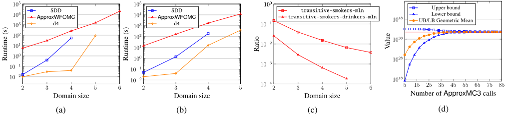
Q1 In Figures 1a and 1b, we show how the domain size affects the runtime of ApproxWFOMC and compare it to the SDD library [Choi and Darwiche, 2013] and the DecisionDNNF compiler d4 [Lagniez and Marquis, 2017]. Note that a small increase in domain size makes the resulting inference problem significantly harder, as the number of Boolean random variables in the joint distribution grows quadratically. Although SDDs outperform ApproxWFOMC at small domain sizes (d = 2, 3 and 4), ApproxWFOMC performs better with larger domains, with SDD compilation running out of memory already with a domain of size 5 on both networks. d4 was more resilient, and is able to handle domains of size up to 5 (but no higher) in the smokers network, and all domain sizes we tested up to 5 in the smokers-drinkers network. We also tried to experiment with WeightMC but the tilt parameter (cf. Section 2.3) was so high that it rendered WeightMC unusable beyond a domain of size 2.

Q2 In Figure 1c, we show the efficiency gain of ApproxWFOMC over using a na¨ıve decomposition of the form in Theorem 2, by quantifying the ratio between the number of FOMC oracle calls made by ApproxWFOMC to the number needed in the decomposition. In both networks the "efficiency ratio" improves significantly as domain size increases, showing that the heuristic-guided search becomes increasingly effective in finding dense regions in the space of weighted models.

Q3 In Figure 1d, we measure how quickly ApproxWFOMC converges to the true WFOMC for a representative domain size d = 4. The bounds rapidly approach a value near that of the true WFOMC (indicated by the red dashed line), meaning that most ApproxMC3 calls are made when the bounds are already relatively close to convergence. This suggests that ApproxWFOMC is well-suited to obtaining rough bounds very quickly (corresponding to large values of τ).

5 Conclusion

We introduced ApproxWFOMC, an anytime approximate WFOMC algorithm with PAC guarantees, and showed how it can be applied to inference in first-order probabilistic models. Results show that it is able to scale to domain sizes that are too large for existing exact methods. Other approximate methods such as MCMC either need exponential time to converge, or are used in practice in such a way that does not guarantee convergence to the stationary distribution (and can therefore give drastically incorrect results). Our method is somewhere in between these: it comes with guarantees, and scales beyond what exact methods can do. Even though a lot of future work is needed before methods like ours bring us efficient inference in large domains, we believe that this paper is an important first step in that direction. There are still several avenues for further research, including tighter integration between the cardinality constraints and ApproxMC3, and application of our method to inference in other statistical relational learning systems such as ProbLog [Fierens et al., 2015].

Acknowledgements

TvB's work is supported by the Research Foundation - Flanders (grant G095917N). OK's work is supported by the OP VVV project CZ.02.1.01/0.0/0.0/16 019/0000765 "Research Center for Informatics" and a donation from X-Order Lab. Part of this work was done while OK was already supported by the Czech Science Foundation project "Generative Relational Models" (20-19104Y).