Learning Bayesian Networks Under Sparsity Constraints: A Parameterized Complexity Analysis

1 Introduction

Bayesian networks are graphical models for probability distributions in which the presence of conditional dependencies between a set of random variables are represented via a directed acyclic graph (DAG) D = (N,A) over a set N of n random variables [Darwiche, 2009]. An arc (u, v) in a Bayesian network means that the distribution of v depends on the value of u. Once we have obtained a Bayesian network, one may infer the distribution of some random variables given the values of other random variables.

First, however, one needs to learn the network from observed data. An important step herein is to learn the structure of the network, that is, the arc set of the network. In this step, one is given for each network vertex v and each set of possible parents of v a parent score and the goal is to learn an acyclic network with a maximal sum of parent scores. To represent the observed data as closely as possible it may seem appropriate to learn a tournament, that is, a DAG in which every pair of vertices u and v is connected either by the arc (u, v) or by the arc (v, u). There are, however, several reasons why learning a tournament-like DAG should be avoided (see [Darwiche, 2009] for a detailed discussion): First, such a network gives no information about which variables are conditionally independent. Second, including too many dependencies in the model makes the model vulnerable to overfitting. Finally, the problem of inferring distributions on a given Bayesian network is intractable when the DAG is tournament-like. More precisely, the inference problem on Bayesian networks is NP-hard [Cooper, 1990]. The key to obtaining efficient inference algorithms is to exploit that the network is tree-like: If the moralized graph has small treewidth, the inference task can be solved more efficiently [Darwiche, 2009]; the moralized graph of a network D is the undirected graph on the same vertex set that is obtained by adding an edge between each pair of vertices that is adjacent or has a common child in D.

∗Contact Author

Motivated by these reasons for avoiding tournament-like networks and instead aiming for tree-like networks, it has been proposed to learn optimal networks under structural constraints that guarantee that the network or its moralized graph is tree-like [Elidan and Gould, 2008; Korhonen and Parviainen, 2013; 2015; Chow and Liu, 1968; Gaspers et al., 2015]. We continue this line of research, focusing on exact algorithms with worst-case running time guarantees. In other words, we want to find out for which structural constraints there are fast algorithms for learning optimal Bayesian networks under these constraints and for which constraints this is presumably impossible.

1.1 Known Results

The problem of learning a Bayesian network without structural constraints, which we call VANILLA-BNSL, is NPhard [Chickering, 1995] and can be solved in 2nnO(1) time by dynamic programming over all subsets of N [Ott and Miyano, 2003; Silander and Myllym¨aki, 2006].

When the network is restricted to be a branching, that is, a directed tree in which every vertex has indegree at most one, then an optimal network can be computed in polynomial time [Chow and Liu, 1968; Gaspers et al., 2015]. Note that learning a more restricted Bayesian network is not necessarily easier: While learning a branching is solvable in polynomial time, the problem becomes NP-hard if we aim to learn a directed path [Meek, 2001].

On the negative side, the BOUNDED-TW-BNSL problem, where the moralized graph of the network is restricted to have treewidth at most ω is NP-hard for every fixed ω ≥ 2 and can be solved in 3nnω+O(1) time [Korhonen and Parviainen, 2013]. Finally, BOUNDED-VC-BNSL where the moralized graph is restricted to have a vertex cover of size at most k can be solved in 4k · n2k+O(1) time [Korhonen and Parviainen, 2015]; a vertex cover in a graph G is a vertex set S such that every edge of G has at least one endpoint in S. Since having a bounded vertex cover implies that the graph has bounded treewidth, the networks that are learned by BOUNDED-VCBNSL allow for fast inference algorithms. An algorithm with running time f(k) · |I|O(1) is unlikely for BOUNDEDVC-BNSL, since BOUNDED-VC-BNSL is W[1]-hard with respect to the parameter k [Korhonen and Parviainen, 2015]. Here, |I| denotes the total input size. In other words, it seems necessary that the degree of the running time polynomial depends on k.

1.2 Our Results

The results for BOUNDED-VC-BNSL [Korhonen and Parviainen, 2015] form the starting point for our work. An alternative view of vertex covers is as follows: A graph has a vertex cover of size k if and only if it can be transformed into an edgeless graph by k vertex deletions. Thus, in BOUNDEDVC-BNSL we learn a network whose moralized graph is close, in terms of the number of vertex deletions, to a sparse graph class. We investigate whether there are further positive examples for such constrained network learning problems.

First, we consider the constraint that the moralized graph can be transformed into a graph with maximum degree 1 by at most k vertex deletions. We show that under this constraint, one can learn an optimal network in nO(k2 ) · |I|O(1) time and thus in polynomial time for every constant value of k. This extends the result for BOUNDED-VC-BNSL in the following sense: the value of k can be arbitrarily smaller than the vertex cover number and thus for fixed k our algorithm can learn an optimal network for a larger class of graphs than the algorithm for BOUNDED-VC-BNSL. Observe that the moralized graphs still have bounded treewidth and thus inference on the learned networks will still be solvable efficiently.

We then show that it is unlikely that this positive result can be improved much further. First, we show that an algorithm with running time f(k) · |I|O(1) is unlikely. Moreover, we show that learning an optimal network that has maximum degree 2 is NP-hard and that learning an optimal network in which every component has at most three vertices is NP-hard (in a graph with maximum degree one every connected component has at most two vertices).

We further extend these negative results by showing that even in the very restricted scenario where we aim to compute an optimal network whose moralized graph has at most k edges, an f(k) · |I|O(1) -time algorithm is unlikely. In contrast, if we restrict instead the number of arcs in the network, we obtain an algorithm with a running time of 2O(k) · |I|O(1) .

Thus, putting structural constraints on the moralized graph may make the problem much harder than putting similar structural constraints on the network itself. We obtain a further hardness result for VANILLA-BNSL: Under standard assumptions in complexity theory, it is impossible that we can transform a given instance of VANILLA-BNSL in polynomial time to an equivalent one of size nO(1) . Thus, it is sometimes necessary to keep an exponential number of parent scores to compute an optimal network.

2 Preliminaries

2.1 Notation

We consider directed and undirected graphs that do not contain multiple edges.

A directed graph D = (N,A) consists of a vertex set N and an arc set A ⊆ N ×N. Let D = (N,A) be a directed graph. If D does not contain directed cycles, then D is called directed acyclic graph (DAG). An arc (u, v) ∈ A is called incoming arc into v and an arc (v, u) ∈ A is called outgoing arc from v. A vertex without incoming arcs is a source. A vertex without outgoing arcs is a sink. The set P A v := {u ∈ N | (u, v) ∈ A} is called parent set of v. The vertices in P A v are called parents of v and for every u ∈ P A v , the vertex v is called child of u. We call v1 an ancestor of vℓ and vℓ a descendant of v1 if there is a path (v1, v2, . . . , vℓ) in D.

An undirected graph G = (V, E) consists of a vertex set V and an edge set E ⊆ {{u, v} | u, v ∈ V }. For a vertex v ∈ V , we write NG(v) := {u | {u, v} ∈ E} to denote the neighborhood of v in G. The degree of a vertex v is defined as degG(v) := |NG(v)|. Given an edge-set E′ ⊆ E, we let G\E′ denote the graph we obtain after deleting the edges in E′ from G. Given a vertex-set V ′ ⊆ V , we let G- V ′ denote the graph we obtain after deleting the vertices in V ′ and their incident edges fromG. A set S ⊆ V is called dissociation set, if G- S has maximum degree one. The size of the smallest possible dissociation set for G is called dissociation number of G.

A graph class Π is a set of undirected graphs. For a graph class Π and k ∈ N, let Π + kv denote the class of graphs that can be transformed into a graph in Π by performing at most k vertex deletions. Analogously, we define Π + ke as the class of graphs that can be transformed into a graph in Π by performing at most k edge deletions. We call Π monotone if Π is closed under edge- and vertex deletions. Note that Π being monotone implies that for every k ∈ N0, the graph classes Π + kv and Π + ke are monotone.

2.2 Bayesian Network Structure Learning

Given a vertex set N, we call a family F = {fv : 2N\{v} → N0 | v ∈ N} a family of local scores for N. Intuitively, for a vertex v ∈ N and some P ∈ 2N\{v} , the value fv(P) ∈ N0 represents the score we obtain if we choose exactly the vertices of P as parents for v. Given a vertex set N, local scores F, and some integer t ∈ N0, an arc set A ⊆ N × N is called (N, F, t)-valid if (N, A) is a DAG and ∑v∈N fv(P A v ) ≥ t.

Given a directed graph D = (N,A), we call the undirected graph M(D) := (V,E1 ∪ E2) with V :=

N, E1 = {{u, v} | (u, v) ∈ A}, and E2 = {{u, v} | u and v have a common child in D} the moralized graph of D. The edges in E2 are called moral edges. We may now define the problem.

(Π + v)-BAYESIAN NETWORK STRUCTURE LEARNING ((Π+ v)-BNSL)

Input: A set of vertices N, local scores F = {fv | v ∈ N}, and two integers t, k ∈ N0.

Question: Is there an (N,F, t)-valid arc set A ⊆ N × N such that M((N, A)) ∈ Π + kv?

Intuitively, (Π + v)-BNSL can be seen as a version of VANILLA-BNSL where we add an additional constraint to the moralized graph of the resulting network. The problem (Π + e)-BNSL is defined on the same input and we ask if there exists an (N, F, t)-valid arc set A such that (N, A) ∈ Π+ ke. For both problems we call the requested arc set A a solution of the instance (N, F, t, k). Note that, if Π is monotone, contains infinitely many graphs, and k = n2 , the property M((N, A)) ∈ Π + kv or M((N, A)) ∈ Π + ke always hold, since every edgeless graph and an empty graph belong to Π. Hence, (Π + v)-BNSL and (Π + e)-BNSL are generalizations of VANILLA-BNSL and thus NP-hard for every monotone and infinite Π. For formal reasons, the problems are stated as decision problems. However, the algorithms presented in this work solve the corresponding optimization problem within the same running time.

Throughout this work, we let n := |N| denote the number of vertices given in an instance I = (N, F, t, k) of (Π + v)- BNSL or (Π+ e)-BNSL. Furthermore, we assume that the local scores F are given in non-zero representation [Ordyniak and Szeider, 2013], that is, for every fv ∈ F, each value fv(P) is only given if it is different from zero. We assume that for N = {v1, . . . , vn}, the local scores F are given as a two-dimensional array F := [Q1,Q2, . . . ,Qn], where each Qi is an array containing all triples (fvi (P), |P|, P) where fvi (P) > 0. The size |F| is then defined as the number of bits we need to store this two-dimensional array. As the size of I we define |I| := n + |F| + log(t) + log(k).

In this work, we consider (Π + v)-BNSL and (Π + e)- BNSL for some monotone graph classes Π. Observe that in these cases the following holds.

Proposition 1 Let Π be a monotone graph property, and let (N, F, t, k) be a yes-instance of (Π+v)-BNSL (or (Π+ e)-BNSL). Then, there exists a solution A for (N,F, t, k) such that for every v ∈ N it holds that fv(P A v ) = 0 implies P A v = ∅.

Given an instance I := (N,F, t, k) and some v ∈ N, we define the set of potential parents of v by PF(v) := {P ⊆ N \{v} : fv(P) > 0}∪{∅}, which are exactly the parent sets stored in F together with the empty set. If Π is monotone, we can assume by Proposition 1 that in a solution A for I, every v has a parent set P A v ∈ PF(v). An important measurement for the running times of our algorithms is the maximum number of potential parent sets δF := maxv∈N |PF(v)| [Ordyniak and Szeider, 2013]. Given a vertex v ∈ N, we can iterate over all vertices in potential parent sets of v in O(δF · n) time.

Another tool for designing algorithms for BNSL problems is the superstructure [Ordyniak and Szeider, 2013]. The superstructure of N and F is the directed graph S ⃗F = (N, AF ) with AF = {(u, v) | ∃P ∈ PF(v) : u ∈ P}.

2.3 Parameterized Complexity

A problem is called slicewise polynomial (XP) for a parameter k if it can be solved in time O(|I|f(k) ) for a computable function f. That is, the problem is solvable in polynomial time when k is constant. A problem is called fixedparameter tractable (FPT) for a parameter k if it can be solved in time f(k) · |I|O(1) for a computable function f. If a problem is W[1]-hard then it is assumed to be fixed-parameter intractable. A problem has a polynomial kernel for a parameter k if there is a polynomial-time algorithm that, given an instance I with parameter k, computes an equivalent instance I ′ with parameter k′ ≤ k of size g(k) where g is a polynomial. For a detailed introduction into parameterized complexity we refer to [Cygan et al., 2015].

3 Vertex Deletion Distances

Let Π1 := {G | G has maximum degree 1}, that is, every G ∈ Π1 consists only of isolated edges and isolated vertices. Observe that Π1 is monotone. In this section we consider (Π1 + v)-BNSL. Note that, given some k ∈ N, a DAG D = (N, A) with M(D) ∈ Π1 + kv is a DAG whose moralized graph has a dissociation set of size at most k. Since the treewidth of a graph is never bigger than the dissociation number plus one, the moralized graph of the resulting Bayesian network has treewidth at most k + 1. Before we describe the main idea of the algorithm we provide the following simple observation .

Proposition 2 Let D = (N, A) be a DAG and S ⊆ N be a dissociation set of M(D). Then, at most 2|S| vertices in N \ S have descendants in S.

The idea is the following: If we know the dissociation set S, all their ancestors Q under A, and the arcs between them, the remaining arcs of A can be found in polynomial time. We start with the following .

Definition 3 let N be a vertex set and let S ⊆ N. A set Q ⊆ N \ S together with an arc-set AQ ⊆ (S ∪ Q) × (S ∪ Q) is called ancestor tuple for S, if

1. DQ := (S ∪Q,AQ) is a DAG, and
2. for every v ∈ Q exists some w ∈ S such that w is a descendant of v in DQ, and
3. in the moralized graph M(DQ), every v ∈ Q has at most one neighbor outside S.

Intuitively, the ancestor tuple 〈Q,AQ〉 is the part of the solution that our algorithm finds via bruteforce. We next formally define an arc set containing the remaining arcs of a solution. To this end, we introduce some notation. Given an ancestor tuple 〈Q, AQ〉 of some S ⊆ N, we let R := N \ (S ∪ Q) denote the remaining vertices of N. Moreover, we define Q0 := {v ∈ Q | degM(DQ)-S(v) = 0} and Q1 := Q\Q0. By Definition 3 c), the vertices of Q1 are the vertices that have degree one in M(DQ) - S.

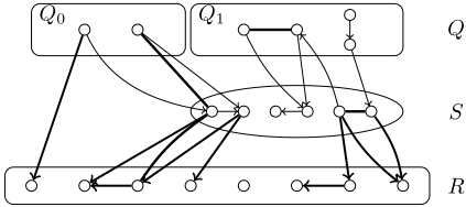
Definition 4 Let N be a vertex set, let S ⊆ N, and let 〈Q,AQ〉 be an ancestor tuple of S. An arc-set AR ⊆ (S ∪ Q0 ∪ R) × R is called suitable for 〈Q, AQ〉 if AR contains no self-loops, and every w ∈ Q0 ∪ R has at most one incident arc in AR ∩ ((R ∪ Q0) × R).

Next, we state the connection between Definitions 3, 4, and DAGs whose moralized graph has dissociation set S. First, an ancestor tuple for some S and a suitable arc set can be combined to a DAG where S is a dissociation set of the moralized graph.

Proposition 5 Let N be a vertex set, let S ⊆ N, let 〈Q, AQ〉 be an ancestor tuple of S, and let AR ⊆ (S ∪Q0 ∪R)×R be a suitable arc set for 〈Q, AQ〉. Then, 1) D := (N, AQ ∪AR) is a DAG, and 2) S is a dissociation set of M(D).

Conversely, the arc set of every DAG whose moralized graph has a dissociation set S can be partitioned into the arc set of an ancestor tuple for S and a suitable arc set; Figure 1 shows an example.

Proposition 6 Let D = (N,A) be a DAG, let S ⊆ N be a dissociation set of M(D). Then, 〈Q, AQ〉 defined by

is an ancestor tuple of S with |Q| ≤ 2|S| and A \ AQ is suitable for 〈Q,AQ〉.

Next, we use ancestor tuples and suitable arc sets to decompose the local scores in (Π1 + v)-BNSL. Let (N, F, t, k) be an instance of (Π1 +v)-BNSL and let S ⊆ N. Furthermore, let 〈Q, AQ〉 be an ancestor tuple for S and let AR be suitable for 〈Q,AQ〉. Then, we set A := AQ ∪ AR and by Proposition 5, D := (N,A) is a DAG and S is a dissociation set of M(D). Observe that all arcs in AR have endpoints in R and all arcs in AQ have endpoints in Q ∪ S. Hence, for every v ∈ N it holds that either all incoming arcs are in AQ or in AR. Hence, the score of A under F is

We next show that, if S and 〈Q,AQ〉 are given, we can find AR in polynomial time. More precisely, we solve the following problem.

(Π1 + v)-BNSL-COMPLETION

Input: A set of vertices N, a subset S ⊆ N, an ancestor tuple 〈Q,AQ〉 for S, local scores F = {fv | v ∈ N}, and an integer t.

Question: Is there an arc-set AR that is suitable for 〈Q, AQ〉 such that ∑v∈R fv(P AR v ) ≥ t?

Proposition 7 (Π1+v)-BNSL-COMPLETION can be solved in O(n2 · (nδF + √n)) time.

PROOF We give a polynomial-time reduction to MAXIMUM WEIGHT MATCHING, where one is given a graph G = (V,E), edge-weights ω : E → N, and ℓ ∈ N and the question is if there exists a set M ⊆ E of pairwise non-incident edges such that ∑e∈M ω(e) ≥ ℓ.

Construction: Let I := (N, S, 〈Q,AQ〉,F, t) be an instance of (Π1 + v)-BNSL-COMPLETION. We construct an equivalent instance (G, ω, ℓ) of MAXIMUM WEIGHT MATCHING. We first define G := (V,E) with V := Q0 ∪ R ∪ R′ , where R′ := {v′ | v ∈ R}, and E := X ∪ Y ∪ Z, where

Next, we define edge-weights ω : E → N: For e = {v, v′ } ∈ Z, we set ω(e) := maxS′⊆S fv(S′ ). Furthermore, for e = {v, w} ∈ Y with v ∈ R and w ∈ Q0, we set ω(e) := maxS′⊆S fv(S′ ∪ {w}). Finally, for e = {v,w} ∈ X, we set ω(e) := max(ϕ(v, w), ϕ(w, v)), where

To complete the construction , we set ℓ := t.

Due to lack of space, the correctness proof is deferred. We provide some intuition: A maximum weight matching M in G corresponds to the parent sets of vertices in R and therefore to arcs in AR. An edge {v, v′ } ∈ Z with v ∈ R corresponds to a parent set of v that contains only vertices from S. Moreover, an edge {v,w} ∈ Y with v ∈ R corresponds to a parent set of v that contains w ∈ Q0 and vertices from S. Finally, an edge {v,w} ∈ X means that either v ∈ P AR w or w ∈ P AR v . Since M is a matching, the corresponding arc set is suitable for 〈Q,AQ〉. ✷

Theorem 8 (Π1 + v)-BNSL can be solved in O((nδF)3k · poly(|I|)) time.

PROOF (SKETCH) Iterate over all possible choices for S and 〈Q,AQ〉 where |S| ≤ k and |Q| ≤ 2k in O((nδF)3k ) time and find the remaining arcs in polynomial time using Proposition 7. ✷

Note that in a Bayesian network whose moralized graph has a dissociation set of size k the maximum parent set size is k+1. Otherwise, the moralized graph has a clique of size at least k +3, contradicting the fact that it has a dissociation set of size k. Hence, we can delete every triple (fv(P), |P|, P) with |P | > k + 1 from F. Afterwards, δF ≤ ( n k+1).

Corollary 9 (Π1 + v)-BNSL can be solved in nO(k2 ) + poly(|I|) time.

We complement the algorithm for (Π1 + v)-BNSL by several hardness results. First, there is little hope to obtain an FPT algorithm for (Π1 + v)-BNSL parameterized by k + t since the problem is W[1]-hard. Observe that this is not implied by the W[1]-hardness of BOUNDED-VC-BNSL since (Π1 + v)-BNSL is a different problem where we aim to find a Bayesian network with different restrictions. However, the proof is closely related to the W[1]-hardness-proof for BOUNDED-VC-BNSL [Korhonen and Parviainen, 2015].

Proposition 10 (Π1+v)-BNSL is W[1]-hard for k+t, even when the superstructure S ⃗F is a DAG and the maximum parent set size is three.

We next consider monotone graph classes that are related to the class Π1 . Let Π2 be the class of graphs that have maximum degree two, and let ΠCOC 3 be the class of graphs where each connected component has size at most three. These graph classes are superclasses of Π1, that is Π1 ⊆ Π2 and Π1 ⊆ ΠCOC 3 . Consequently, if a graph G belongs to the graph class Π1+kv for some k ∈ N0, then there exist k′ ≤ k and k′′ ≤ k such that G ∈ Π2 + k′ v and G ∈ ΠCOC 3 + k′′ v. Moreover, observe that the treewidth of G is not bigger than min(k′ , k′′ ) + O(1).

With the next proposition we show that there is little hope that we can solve (Π2 + v)-BNSL or (ΠCOC 3 + v)-BNSL in XP time when parameterized by k. The hardness of (Π2+v)- BNSL relies on the fact that learning paths is NP-hard [Meek, 2001].

Proposition 11 (Π2+v)-BNSL and (ΠCOC 3 +v)-BNSL are NP-hard even if k = 0.

4 Edge Deletion Distances

4.1 Bounded-Edges-BNSL

We now consider a version of BNSL, where we aim to learn a network whose moralized graph has a bounded number of edges. More precisely, we consider (Π0 + e)-BNSL where Π0 is the class of edgeless graphs. Clearly, Π0 is monotone and (Π0 + e)-BNSL can be solved in O(n2k · poly(|I|)) time by a brute-force algorithm. To put this into context, we show that there is little hope to solve (Π0 + e)- BNSL in FPT time for t + k.

Theorem 12 (Π0 + e)-BNSL is W[1]-hard when parameterized by t + k, even when S⃗F is a DAG and the maximum parent set size is three.

Learning a Bayesian network whose moralized graph has a bounded feedback edge set is also W[1]-hard when parameterized by the size of the feedback edge set. More formally, let ΠF be the class of forests, which are undirected acyclic graphs.

Theorem 13 (ΠF + e)-BNSL is W[1]-hard when parameterized by k, even when S⃗F is a DAG and the maximum parent set size is four.

For efficient inference it is desirable to have a small treewidth in the moralized graph. The size of a feedback edge set is a large upper bound for the treewidth. Since even learning Bayesian networks under this constraint is W[1]-hard, it appears to be unlikely to obtain fixed-parameter tractability for natural parameters that bound the treewidth of the moralized graph.

4.2 Bounded-Arcs-BNSL

Next, we consider a version of BAYESIAN NETWORK STRUCTURE LEARNING where we want to learn a Bayesian network with a bounded number of arcs. In contrast to (Π0 + e)-BNSL, the additional sparsity constraint does not affect the moralized graph but only the arcs of the DAG itself. The problem is formally defined as follows.

BA-BNSL

Input: A set of vertices N, local scores F = {fv | v ∈ N}, and two integers t, k ∈ N.

Question: Is there an (N, F, t)-valid arc set A ⊆ N × N such that |A| ≤ k?

BA-BNSL is a generalization of VANILLA-BNSL and therefore NP-hard. We prove that BA-BNSL becomes polynomial-time solvable if the superstructure is a DAG. The algorithm uses dynamic programming over a topological ordering of S ⃗F .

Proposition 14 BA-BNSL can be solved in O(δF · k · n) time if the superstructure S⃗F is a DAG.

PROOF We give a simple dynamic programming algorithm. Let N := {1, . . . , n}, and let (N,F, t, k) be an instance of BA-BNSL such that S⃗F is a DAG. Then, there exists such a topological ordering of S ⃗F . Without loss of generality, let (n, n - 1, . . . , 2, 1) be such topological ordering. Hence, for every arc (a, b) of S⃗F it holds that a > b.

The dynamic programming table T has entries of the type T[i, j] for all i ∈ {0, 1, . . . , n} and j ∈ {0, 1, . . . , k}. Each entry stores the maximum sum of local scores of the vertices (i, . . . , 1) of the topological ordering that can be obtained by an arc set A of size at most j. For i = 0, we set T[0, j] = 0 for all j ∈ {0, . . . , k}. The recurrence to compute an entry for i > 0 is

and the result can then be computed by checking if T [n, k] ≥ t. The corresponding network can be found by traceback. The correctness proof is straightforward and thus omitted. The size of T is O(n · k) and each entry T[i, j] can be computed in O(δF) time by iterating over the at most δF triples (fi(P), |P|, P) in F for the vertex i. Therefore, BABNSL can be solved in O(δF · k · n) time if S⃗F is a DAG. ✷

4.3 ARandomized Algorithm for BA-BNSL

The dynamic programming algorithm behind Proposition 14 can be adapted to obtain an FPT algorithm for BA-BNSL when parameterized by the number of arcs k. The algorithm is based on color coding [Alon et al., 1995]: In a Bayesian network with at most k arcs, there are at most 2k vertices which are endpoints of such arcs. The idea of color coding is to randomly color the vertices of N with 2k colors and find a solution A where all vertices that are incident with arcs of A are colored with pairwise distinct colors. To describe the color coding algorithm, we introduce some notation. Let N be a set of vertices. A function χ : N → {1, . . . , 2k} is called a coloring (of N with 2k colors). Given a color c ∈ {1, . . . , 2k}, we call χ-1 (c) := {v ∈ N | χ(v) = c} the color class of c. For a subset N ′ ⊆ N, we let χ(N ′ ) := {χ(v) | v ∈ N ′ }, and for a subset C ⊆ {1, . . . , 2k} we let χ-1 (C) := ⋃c∈C χ-1 (c). The following definition is important for our algorithm.

Definition 15 Let N be a set of vertices and let χ : N → {1, . . . , 2k} be a coloring of N. An arc set A ⊆ N × N is called color-loyal for χ if for every color class χ-1 (c) it holds that

1. there is no (v,w) ∈ A with v,w ∈ χ-1 (c), and
2. there is at most one vertex v ∈ χ-1 (c) such that P A v ̸= ∅.

Consider the following auxiliary problem.

COLORED BA-BNSL

Input: A set of vertices N, local scores F = {fv | v ∈ N}, two integers t, k ∈ N, and a coloring χ : N → {1, . . . , 2k}.

Question: Is there an (N, F, t)-valid arc set A ⊆ N × N that is color-loyal for χ and |A| ≤ k?

Intuitively, COLORED BA-BNSL is the problem that we solve after we randomly choose a coloring of N. The correspondence between BA-BNSL and COLORED BA-BNSL is as follows.

Proposition 16 Let I = (N,F, t, k) be an instance of BABNSL. If I is a yes-instance of BA-BNSL, then there exist at least (2k)!(2k)(n-2k) colorings χ : N → {1, 2, . . . , 2k} such that (N, F, t, k, χ) is a yes-instance of COLORED BABNSL.

Proposition 17 COLORED BA-BNSL can be solved in O(4k k2n2 δF) time.

PROOF We fill a dynamic programming table T with entries of type T [C ′ , k′ ] where C ′ ⊆ C and k′ ∈ {0, 1, . . . , k}. Every entry stores the maximum value of ∑v∈χ-1 (C′ ) fv(P A v ) over all possible DAGs D = (N, A), where A ⊆ χ-1 (C ′ ) × χ-1 (C ′ ) is color-loyal for χ and contains at most k′ arcs. We set T[{c}, k′ ] := ∑w∈χ-1 (c) fw(∅) for every c ∈ C and k′ ∈ {0, 1, . . . , 2k}. The recurrence to compute the entry for C ′ ⊆ C with |C ′ | > 1 is

where

The result can be computed by checking if T [C, k] ≥ t. Note that the corresponding network can be found via traceback.

The correctness proof is straightforward and thus omitted. The size of T is O(22k · k). We omit the proof of the polynomial running time part. ✷

Propositions 16 and 17 give the following.

Theorem 18 There exists a randomized algorithm for BABNSL that, in time O((2e)2k · k2n2 δF) returns no, if given a no-instance and returns yes with a constant probability of at least 1 - 1e , if given a yes-instance.

The algorithm can be derandomized with standard techniques [Naor et al., 1995; Cygan et al., 2015].

Corollary 19 BA-BNSL can be solved in (2e)2k ·kO(log(k)) · poly(|I|) time.

Bounding the number of arcs appears to be not so relevant for practical use. However, the algorithm might be useful as a heuristic upper-bound: If we want to add a restricted number of dependencies to a given Bayesian network, the result of BA-BNSL gives an upper bound for the profit we can expect from that modification. The above algorithm is complemented by the following negative result.

Theorem 20 BA-BNSL parameterized by t + k does not admit a polynomial kernel unless NP ⊆ coNP/poly even when k = n2 .

Observe that for instances of BA-BNSL with k = n2 , the budget of arcs can never be exceeded since a DAG has at most (n2 ) < n2 arcs. Hence, on instances with k = n2 we ask for an (N,F, t)-valid arc set without additional sparsity constraints. Thus, BA-BNSL and VANILLA-BNSL are the same when k = n2 . Then, Theorem 20 implies the following.

Corollary 21 VANILLA-BNSL parameterized by n does not admit a polynomial kernel unless NP ⊆ coNP/poly.

5 Conclusion

We have outlined the tractability borderline of BAYESIAN NETWORK STRUCTURE LEARNING with respect to several structural constraints on the learned network or on its moralized graph. In particular, we have shown that putting structural sparsity constraints on the moralized graph may make the problem harder than putting similar constraints on the network. This is somewhat counterintuitive since the moralized graph is a supergraph of the underlying undirected graph of the network. It seems interesting to investigate this issue further, that is, to find structural constraints such that putting these constraints on the network leads to an easier problem than putting them on the moralized graph.

While none of our algorithms have direct practical applications, they may be useful as bounds on the score that can be achieved for example by adding k arcs to a network that is currently considered in the search. Thus, it would be interesting to explore variants of BAYESIAN NETWORK STRUCTURE LEARNING where the input contains a partial network and the aim is to extend it. Do the positive results for BAYESIAN NETWORK STRUCTURE LEARNING also hold for this more general problem?