
Cost-Partitioned Merge-and-Shrink Heuristics for Optimal Classical Planning
Proceedings of the Twenty-Ninth International Joint Conference on Artificial Intelligence. Main track. Pages 4152-4160.
https://doi.org/10.24963/ijcai.2020/574
Keywords
- Heuristic Search and Game Playing: Heuristic Search
- Planning and Scheduling: Planning Algorithms
- Planning and Scheduling: Search in Planning and Scheduling
Abstract
Cost partitioning is a method for admissibly combining admissible heuristics.
In this work, we extend this concept to merge-and-shrink (M&S) abstractions
that may use labels that do not directly correspond to operators. We
investigate how optimal and saturated cost partitioning (SCP) interact with
M&S transformations and develop a method to compute SCPs during the
computation of M&S. Experiments show that SCP significantly improves M&S on
standard planning benchmarks.
- [Bäckström and Nebel, 1995] Christer Bäckström and Bern- hard Nebel. Complexity results for SAS + planning. Com- putational Intelligence, 11(4):625-655, 1995.
- [Dräger et al., 2009] Klaus Dräger, Bernd Finkbeiner, and Andreas Podelski. Directed model checking with distance- preserving abstractions. International Journal on Software Tools for Technology Transfer, 11(1):27-37, 2009.
- [Edelkamp, 2001] Stefan Edelkamp. Planning with pattern databases. In Amedeo Cesta and Daniel Borrajo, editors, Proceedings of the Sixth European Conference on Plan- ning (ECP 2001), pages 84-90. AAAI Press, 2001.
- [Ghallab et al., 2004] Malik Ghallab, Dana Nau, and Paolo Traverso. Automated Planning: Theory and Practice.
- Morgan Kaufmann, 2004.
- [Hart et al., 1968] Peter E. Hart, Nils J. Nilsson, and Bertram Raphael. A formal basis for the heuristic determination of minimum cost paths. IEEE Transactions on Systems Science and Cybernetics, 4(2):100-107, 1968.
- [Helmert et al., 2014] Malte Helmert, Patrik Haslum, Jörg Hoffmann, and Raz Nissim. Merge-and-shrink abstrac- tion: A method for generating lower bounds in factored state spaces. Journal of the ACM, 61(3):16:1-63, 2014.
- [Helmert, 2006] Malte Helmert. The Fast Downward plan- ning system. Journal of Artificial Intelligence Research, 26:191-246, 2006.
- [Katz and Domshlak, 2010] Michael Katz and Carmel Domshlak. Optimal admissible composition of abstraction heuristics. Artificial Intelligence, 174(12-13):767-798, 2010.
- [Nissim et al., 2011] Raz Nissim, Jörg Hoffmann, and Malte Helmert. Computing perfect heuristics in polynomial time: On bisimulation and merge-and-shrink abstraction in opti- mal planning. In Toby Walsh, editor, Proceedings of the 22nd International Joint Conference on Artificial Intelli- gence (IJCAI 2011), pages 1983-1990. AAAI Press, 2011. IJCAI
- [Pearl, 1984] Judea Pearl. Heuristics: Intelligent Search Strategies for Computer Problem Solving. Addison- Wesley, 1984.
- [Pommerening et al., 2015] Florian Pommerening, Malte Helmert, Gabriele Röger, and Jendrik Seipp. From non-negative to general operator cost partitioning. In Blai Bonet and Sven Koenig, editors, Proceedings of the Twenty-Ninth AAAI Conference on Artificial Intelligence (AAAI 2015), pages 3335-3341. AAAI Press, 2015.
- [Seipp and Helmert, 2018] Jendrik Seipp and Malte Helmert. Counterexample-guided Cartesian abstrac- tion refinement for classical planning. Journal of Artificial Intelligence Research, 62:535-577, 2018.
- [Seipp et al., 2017a] Jendrik Seipp, Thomas Keller, and Malte Helmert. A comparison of cost partitioning algo- rithms for optimal classical planning. In Laura Barbulescu, Jeremy Frank, Mausam, and Stephen F. Smith, editors, Proceedings of the Twenty-Seventh International Con- ference on Automated Planning and Scheduling (ICAPS 2017), pages 259-268. AAAI Press, 2017.
- [Seipp et al., 2017b] Jendrik Seipp, Florian Pommerening, Silvan Sievers, and Malte Helmert. Downward Lab. https: //doi.org/10.5281/zenodo.790461, 2017. DOI
- [Seipp et al., 2020] Jendrik Seipp, Thomas Keller, and Malte Helmert. Saturated cost partitioning for optimal classi- cal planning. Journal of Artificial Intelligence Research, 67:129-167, 2020.
- [Sievers et al., 2014] Silvan Sievers, Martin Wehrle, and Malte Helmert. Generalized label reduction for merge- and-shrink heuristics. In Carla E. Brodley and Peter Stone, editors, Proceedings of the Twenty-Eighth AAAI Confer- ence on Artificial Intelligence (AAAI 2014), pages 2358- 2366. AAAI Press, 2014.
- [Sievers et al., 2016] Silvan Sievers, Martin Wehrle, and Malte Helmert. An analysis of merge strategies for merge-and-shrink heuristics. In Amanda Coles, Andrew Coles, Stefan Edelkamp, Daniele Magazzeni, and Scott Sanner, editors, Proceedings of the Twenty-Sixth Interna- tional Conference on Automated Planning and Scheduling (ICAPS 2016), pages 294-298. AAAI Press, 2016.
- [Sievers et al., 2020a] Silvan Sievers, Florian Pommeren- ing, Thomas Keller, and Malte Helmert. Code, bench- marks and experiment data for the IJCAI 2020 paper "Cost-Partitioned Merge-and-Shrink Heuristics for Opti- mal Classical Planning". https://doi.org/10.5281/zenodo. 3775871, 2020. DOI
- [Sievers et al., 2020b] Silvan Sievers, Florian Pommerening, Thomas Keller, and Malte Helmert. Cost-partitioned merge-and-shrink heuristics for optimal classical plan- ning: Technical report. Technical Report CS-2020-001, University of Basel, Department of Mathematics and Computer Science, 2020.
- [Sievers, 2018] Silvan Sievers. Merge-and-shrink heuristics for classical planning: Efficient implementation and par- tial abstractions. In Vadim Bulitko and Sabine Storandt, editors, Proceedings of the 11th Annual Symposium on Combinatorial Search (SoCS 2018), pages 90-98. AAAI Press, 2018.
References were extracted automatically from the PDF and may contain errors.
Full text extracted automatically from the PDF; figures, tables and equations may differ. The PDF is the version of record.
1 Introduction
Classical planning [Ghallab et al., 2004] aims to find a sequence of actions that leads from an initial world situation to a specified goal. A state-of-the-art approach to optimally solving classical planning problems is A* search [Hart et al., 1968] with an admissible heuristic [Pearl, 1984]. Abstractions are a state-of-the-art class of admissible heuristics and contain the merge-and-shrink (M&S) framework [Dr¨ager et al., 2009; Helmert et al., 2014; Sievers et al., 2014], which repeatedly applies transformations to a given state space.
A common problem of abstractions is that they often contain useful information only for parts of a planning task, while completely ignoring the rest. A possible solution to this problem is the combination of different abstractions admissibly with operator cost partitioning [Katz and Domshlak, 2010; Seipp et al., 2017a], which distributes the operator costs among the abstractions guaranteeing that the sum of their heuristic values is admissible. It has successfully been used with Cartesian abstractions [Seipp and Helmert, 2018] and pattern databases [Edelkamp, 2001], but not yet with M&S.
In this paper, we take a first step towards closing this gap. We transfer the notion of operator cost partitioning to M&S abstractions, thus defining label cost partitionings. We then analyze how the heuristic value of optimal [Katz and Domshlak, 2010; Pommerening et al., 2015] and saturated cost partitioning (SCP) [Seipp and Helmert, 2018] is affected by different M&S transformations. Based on these insights, we present a practical approach that interleaves computing SCPs with the M&S algorithm. An experimental evaluation on standard benchmarks shows that combining M&S heuristics in SCPs significantly improves their performance.
2 Background
2.1 Classical Planning
Although our techniques are applicable to any transition system with a so-called factored structure, we show-case them using classical planning tasks in the SAS+ formalism [B¨ackstr¨om and Nebel, 1995]. Such a task is defined as Π = 〈V,O, cost, s0, s⋆〉. V is a finite set of state variables v, each with a finite domain dom(v). A partial state s is an assignment over vars(s) ⊆ V, mapping each v ∈ vars(s) to a value d ∈ dom(v). It is a state if vars(s) = V. State s satisfies partial state s′ , written s |= s′ , if s(v) = s′ (v) for all v ∈ vars(s′ ). O is a finite set of operators o = 〈preo , effo 〉, where preo and effo are partial states called the precondition and effect of o. The cost function cost : O → R+0 maps each operator to its cost. Finally, s0 is the initial state, and s⋆ a partial state called the goal.
For a state s and operator o with s |= preo the successor state sJoK is defined as sJoK(v) = effo (v) for all v ∈ vars(effo ) and sJoK(v) = s(v) for all other variables. A planning task Π induces a transition system Θ(Π) = 〈S, L, cost, T, sI, SG〉, where S is the set of states over V; L = O are labels with costs cost(ℓ) = cost(o) for ℓ ∈ L; T are the transitions {s ℓ-→ t | s, t ∈ S, ℓ ∈ L, s |= preℓ , t = sJℓK}; sI = s0; and SG = {s ∈ S | s |= s⋆} are the goal states. For a transition system Θ, we write S(Θ) for its set of states.
A solution for a planning task is a plan, i.e. a sequence of labels that induces a path in Θ(Π) from sI to some state in SG. The cost of a plan is the sum of its label costs. Optimal planning aims at finding a plan of minimal cost or proving that no plan exists. To optimally solve planning tasks, we use the A∗ algorithm with admissible heuristics. A heuristic for a transition system Θ with labels L and cost function cost is a function h : S(Θ) → R ∪ {∞} which estimates the cost of reaching a goal state from s in Θ. We write h(s, cost′ ) for the evaluation of h on state s ∈ S(Θ), however using an alternative cost function cost′ instead of cost. A heuristic h is admissible if for all states s ∈ S(Θ), h(s) ≤ h∗ (s), where h∗ (s) is the true cost of reaching a goal state from s.
2.2 Merge-and-Shrink
Merge-and-shrink (M&S) is a framework for computing abstractions of transition systems. An abstraction maps a transition system to a different transition system that preserves all plans but is typically smaller and easier to solve. Formally, an abstraction α of a transition system Θ = 〈S,L, cost, T, sI, SG〉 is a homomorphism defined on the states S of Θ. The induced abstract transition system is defined as α(Θ) = 〈{α(s) | s ∈ S},L, cost, {α(s) ℓ-→ α(t) | s ℓ-→ t ∈ T}, α(sI), {α(s) | s ∈ SG}〉.
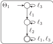
M&S is applicable to transition systems which exhibit a socalled factored structure: a factored transition system (FTS) F = 〈Θ1, . . . ,Θn〉 consists of transition systems Θi (also called factors) sharing the same set of labels and the same cost function. It is a compact ("factored") representation of its product system ⊗ F = 〈S⊗,L, cost, T ⊗, s⊗I , S⊗ G 〉, where S⊗ = ∏ni=1 Si is the Cartesian product of the state sets; there is a transition 〈s1 , . . . , sn 〉 ℓ-→ 〈t1 , . . . , tn 〉 in T ⊗ iff si ℓ-→ ti ∈ T i for all 1 ≤ i ≤ n; the initial state is s⊗I = 〈s1I , . . . , snI 〉; and the set of goal states is S⊗ G = ∏ni=1 SiG . We write S(F) to denote the states of the product of F.
A planning task Π = 〈V,O, cost, s0, s⋆〉 induces the FTS F(Π) consisting of the atomic factors Θv for all variables v ∈ V: Θv is the projection of Π to v, i.e., Θv = 〈dom(v),O, cost, T v , s0[v], SvG〉. The set of transitions T v consists of the transitions s o-→ t for the state s = preo [v] if v ∈ vars(preo ) and for all states s ∈ dom(v) otherwise, and for the state t with t = effo [v] if v ∈ vars(effo ) and t = s otherwise. If v is not mentioned in the goal of Π, all states of Θv are goal states (SvG = dom(v)), otherwise there is a single goal state SvG = {s⋆[v]}.
Figure 1 shows an example FTS F = 〈Θ1, Θ2, Θ3〉. When drawing transition systems, we mark goal states with a double circle and the initial state with an incoming arrow without label. All other arrows are labeled and denote transitions of the transition system. Unless stated otherwise, we assume a constant label cost of 1 (called unit cost).
Starting from any given FTS F = 〈Θ1, . . . ,Θn〉, M&S iteratively applies transformations of F. To do so, it keeps track of the current FTS F ′ , a state mapping Σ : S(F) → S(F ′ ) from states of F to states of F ′ , and a label mapping λ : L → L′ from labels L of F to labels L′ of F ′ . A transformation from F to F ′ specifies F ′ , the state mapping Σ, and the label mapping λ. Applying such a transformation means to replace the current FTS F by F ′ and to compose the maintained mappings with those of the transformation. We consider three transformations of the M&S framework:
Merging. Merging replaces two factors of F, w.l.o.g. Θ1 and Θ2, by their product. Formally: F ′ = 〈Θ1 ⊗ Θ2,Θ3, . . . ,Θn〉, Σ(〈s1, . . . , sn〉) = 〈〈s1, s2〉, s3, . . . , sn〉 (where 〈s1, s2〉 is the product state in Θ1 ⊗ Θ2 that results from the previous states s1 of Θ1 and s2 of Θ2), and λ = id.
Θ2
ℓ1, ℓ2
ℓ1, ℓ2
ℓ1, ℓ2
ℓ3
Θ3
ℓ1, ℓ2
ℓ1, ℓ2
ℓ3
Θ′1
ℓ4
ℓ4
ℓ3
ℓ3
ℓ3, ℓ4
α(Θ′2 )
ℓ3
ℓ4
ℓ4
Θ′2
ℓ4
ℓ4
ℓ4
ℓ3
Θ3
ℓ4
ℓ4
ℓ3
Shrinking. Shrinking applies an abstraction α to one of the factors of F, w.l.o.g. Θ1. Formally: F ′ = 〈α(Θ1),Θ2, . . . ,Θn〉, Σ(〈s1, . . . , sn〉) = 〈α(s1), s2, . . . , sn〉, and λ = id. Shrinking is called h-preserving iff h∗Θ1 (s) = h∗α(Θ1) (α(s)) for all s ∈ S(Θ1).
All three types of transformations guarantee that at any time of the M&S computation, each factor Θi is an abstraction of the original product ⊗ F .
Label reduction. Analogously to shrinking, label reduction applies a homomorphism to the set of labels of F. Formally: λ : L → L′ is the label mapping of the reduction, Σ is the identity mapping, and F ′ = 〈Θ′1 , . . . ,Θ′n 〉, where Θ′i is defined based on Θi = 〈Si ,L, cost, T i , siI , SiG〉 as follows: Θ′i = 〈Si ,L′ , cost′ , {s λ(ℓ) --→ t | s ℓ-→ t ∈ T i }, siI , SiG〉 with cost′ (ℓ′ ) = minℓ∈λ-1 (ℓ′ ) cost(ℓ) for all λ′ ∈ L′ .
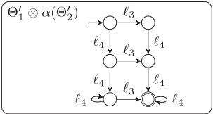
Example 1. Consider the FTS F shown in Figure 1. In a first step, a label reduction transformation λ combines the labels ℓ1, ℓ2 into a new label ℓ4. The resulting transformed FTS F ′ = 〈Θ′1 ,Θ′2 ,Θ′3 〉 is shown at the top of Figure 2.
In a second step, a shrink transformation applies an abstraction α to Θ′2 such that the two gray states are combined. The resulting FTS is F ′′ = 〈Θ′1 , α(Θ′2 ),Θ′3 〉 and the factor α(Θ′2 ) is shown in the bottom left of Figure 2 (the other factors remain unchanged).
Finally, a merge transformation merges Θ′1 and α(Θ′2 ) of F ′′ . The product is shown in the bottom right of Figure 2. The final FTS is F ′′′ = 〈(Θ′1 ⊗ α(Θ′2 )), Θ′3 〉.
In the context of planning, M&S is usually used to compute a heuristic. Let FTS F ′ = 〈Θ1, . . . , Θn〉 and state mapping Σ be the result obtained when executing M&S on some FTS F . We define the factor heuristic hΘi for F as the perfect heuristic for the i-th factor of F ′ : hΘi (s) = h∗Θi (Σ(s)i). Then, the M&S heuristic for F is defined as the maximum over the factor heuristics: hM&S F (s) = max1≤i≤n hΘi (s) for all s ∈ S(F). For the FTS F of Figure 1, we obtain hM&S F (sI) = max(hΘ1 (sI), hΘ2 (sI), hΘ3 (sI)) = max(2, 2, 2) = 2. For the FTS F ′′′ from Example 1, we obtain hM&S F ′′′ (sI) = max(3, 1) = 3.
As mentioned above, all transformations are such that the result is an abstraction. Therefore, hM&S is admissible. Merging is even an exact transformation, i.e., the perfect heuristic values of the product system of the FTSs are unchanged.
Shrinking with abstraction α is not exact in general, but is exact if it combines states according to a bisimulation relation ∼ between states [Nissim et al., 2011]. Such a relation satisfies s ∼ t ("s and t are bisimilar") iff 1) either both s, t are goal states or both are not goal states, and 2) for all s ℓ-→ s′ , there exists t ℓ-→ t′ with s′ ∼ t′ . Shrinking is based on a bisimulation ∼ if α(s) = α(t) iff s ∼ t. It is guaranteed to be h-preserving. The two states combined in Example 1 are not bisimilar for any ∼, and the transformation is not exact.
Label reduction with label mapping λ is also not exact in general, but is exact if there is Θ ∈ F such that for all labels ℓ1, ℓ2 ∈ L with λ(ℓ1) = λ(ℓ2), we have cost(ℓ1) = cost(ℓ2) and ℓ1 and ℓ2 are Θ-combinable [Sievers et al., 2014]. Two labels ℓ1 and ℓ2 are called Θ-combinable if they have parallel transitions in all factors except Θ, i.e., if s ℓ1 -→ t ∈ T ′ iff s ℓ2 -→ t ∈ T ′ for the transitions T ′ of all Θ′ ∈ F \ {Θ}. Labels ℓ1 and ℓ2 combined in Example 1 are Θ1-combinable because they have parallel transitions in Θ2 and Θ3. Since they also have the same cost, the transformation is exact.
To obtain a concrete M&S algorithm, we must decide when to perform which transformation. We follow the literature and define the algorithm as shown in Algorithm 1 in Section 6, for simplicity without showing state and label mappings. (Ignore H, which is related to cost partitioning, discussed later.) The main loop (lines 4-11) runs until the current FTS F ′ only consists of one element or a time limit is reached. One iteration of the loop does the following: decide which two factors Θi,Θj of F ′ to merge in this iteration (line 5), apply exact label reduction (line 6), possibly shrink Θi and/or Θj to respect a size limit (lines 8 and 9), and finally perform the merge (line 10). The algorithm returns hM&S F computed over F ′ (line 12 shows how the extended algorithm computes a cost-partitioned heuristic instead). All transformations are parameterized by so-called transformation strategies.
2.3 Cost Partitioning
Operator cost partitioning [Katz and Domshlak, 2010] allows to admissibly combine admissible heuristics by distributing operator costs among them. Let Π be a planning task with operator costs cost and let H = 〈h1, . . . , hn〉 be admissible heuristics for Π. The cost functions C = 〈cost1, . . . , costn〉 form a cost partition if ∑ni=1 costi ≤ cost. The costpartitioned heuristic hH,C(s) = ∑ni=1 hi(s, costi) is admissible. We discuss two methods to design cost partitions.
Saturated cost partitioning (SCP). The SCP method [Seipp et al., 2020] greedily assigns costs to the heuristics H in a given order ω. To simplify the presentation, we consider the order ω = 〈h1, . . . , hn〉 but in general, ω can be any permutation of the heuristics in H. The algorithm keeps track of a remaining cost function rci which is initialized with the cost function cost, i.e., rc0 = cost. In each step i = 1, . . . , n, the cost function costi is set to a minimal cost function that satisfies hi(s, rci-1) = hi(s, costi) for all s, called the saturated cost function. The remaining cost function is then reduced by costi, i.e., rci = rci-1-costi. In abstraction heuristics where the heuristic value is defined as the cheapest path in a transition system with transitions T, the saturated cost function is unique: costi(o) = maxs o-→t∈T (hi(s, rci-1) - hi(t, rci-1)). The saturated cost partitioning heuristic is defined as hH,C(s) for the discovered cost partition C = 〈cost1, . . . , costn〉.
Optimal cost partitioning (OCP). In contrast to suboptimal cost partitioning methods like SCP, OCP distributes the costs in an optimal way [Katz and Domshlak, 2010]. An OCP for a planning task Π with cost function cost, a state s, and admissible heuristics H = 〈h1, . . . , hn〉 is a cost partition C ∗ = 〈cost1, . . . , costn〉 such that hH,C∗(s) ≥ hH,C(s) for all cost partitions C. The optimal cost partitioning heuristic is defined as hH,C∗(s). Note that C ∗ depends on s, so the heuristic can use a different cost partition in each state. If the heuristics H are abstraction heuristics with induced abstract transition systems Θi = 〈Si ,L, T i , siI , SiG〉, the value hH,C∗(s) is the objective value of the following linear program (LP) or ∞ if the LP is unbounded:
Example 2. Consider the FTS of Figure 1 to be the induced FTS F(Π) of a planning task Π. (Actually, it cannot be, but for simplicity we ignore this subtlety.) The factors are the atomic factors for Π, which are abstractions of Π where each label corresponds to an operator. The corresponding abstraction heuristics H = 〈h1, h2, h3〉 are defined as the shortest path in each abstraction.
To compute the the SCP heuristic of H with ω = H, we first set rc0(ℓi) = 1 for 1 ≤ i ≤ 3. The saturated costs are cost1(ℓ1) = cost1(ℓ2) = 1 and cost1(ℓ3) = 0, and therefore rc1(ℓ1) = rc1(ℓ2) = 0 and rc1(ℓ3) = 1. In the second iteration, we get saturated costs cost2(ℓ1) = cost2(ℓ2) = 0 and cost2(ℓ3) = 1. All remaining costs are 0 now and cost3(ℓi) = 0 for 1 ≤ i ≤ 3. Thus the heuristic value of the SCP heuristic is h1(s0, cost1) + h2(s0, cost2) + h3(s0, cost3) = 2 + 1 + 0 = 3. If we consider the order ω = 〈h2, h1, h3〉 instead, h2 receives all costs and the heuristic value becomes h1(s0, cost1)+h2(s0, cost2)+h3(s0, cost3) = 0+2+0 = 2
An OCP can be computed by solving the LP above. Note that the LP does not exclude negative costs and they are useful here. An optimal solution is cost1(ℓi) = 0 for 1 ≤ i ≤ 3; cost2(ℓ1) = cost2(ℓ2) = 0, cost2(ℓ3) = 3; and cost3(ℓ1) = cost3(ℓ2) = 1, cost3(ℓ3) = -2. The heuristic value of the OCP heuristic is h1(s0, cost1) + h2(s0, cost2) + h3(s0, cost3) = 0 + 3 + 2 = 5.
In the example, we used the fact that there is a one-to-one correspondence between the labels of an induced FTS F(Π) and the operators of Π. However, after performing M&S transformations (in particular label reduction), we lose this correspondence. In the following, we introduce a more general form of cost partitioning, which we then use to discuss cost partitioning on an arbitrary FTS.
3 Label Cost Partitioning
Operator cost partitioning partitions operator cost functions, so it is not directly applicable to factored transition systems with arbitrary labels. However, we can easily lift the notion to general (and in particular to factored) transition systems.
Definition 1. Let cost : L→R+0 be a label cost function for a set of labels L. The cost functions C = 〈cost1, . . . , costn〉 with costi : L → R form a label cost partition if they satisfy ∑ni=1 costi ≤ cost.
Definition 2. Let F = 〈Θ1, . . . ,Θn〉 be an FTS with labels L and a label cost function cost. Let C = 〈cost1, . . . , costn〉 be a label cost partition. The label-cost-partitioned heuristic is hF,C(s) = ∑ni=1 hΘi (s, costi).
Proposition 1. Let Θ be a transition system and let F = 〈Θ1, . . . ,Θn〉 and C be defined as above. If every hΘi is admissible for Θ, then hF,C is an admissible heuristic for Θ.
Proof. The proof is analogous to the one for operator cost partitioning [Pommerening et al., 2015].
As a special case, we can conclude that any label cost partition over the factors of an FTS F created by M&S induces an admissible heuristic: we know that the factor heuristics hΘi are admissible heuristics for the product system of F, which in turn is an abstraction of the original planning task.
As with other cost-partitioned heuristics, there are several methods to compute the partition C. We consider optimal and saturated cost partitioning here and define hOCP F (s) as hF,C∗(s) for a label cost partition C ∗ that is optimal for s, and hSCP F,ω (s) as hF,C(s) for a saturated label cost partition C for s under order ω. Both heuristics are computed analogously to their counterparts for planning tasks. In particular, hOCP F is defined by the LP from Section 2.3 except that L is the set of labels of F . We denote this LP by OCP(F ).
We also consider a more general form of label cost partitioning, where factors of different FTSs are used. We use this to combine factors from different stages of the M&S computation. The main issue with this is that the factors may use different labels. However, for M&S each factor comes from a transformed FTS of a common base FTS (e.g., F(Π)). In such cases, we can treat the combination as a label cost partitioning of the base FTS and translate labels accordingly.
Definition 3. Let L be a set of labels and cost : L →R+0 be a label cost function. For 1 ≤ i ≤ n, let Li be a different set of labels and λi : L→Li a label mapping function.
Then the functions C = 〈cost1, . . . , costn〉 with costi : Li → R form an extended label cost partition if ∑ni=1 costi(λi(ℓ)) ≤ cost(ℓ) holds for all ℓ ∈ L.
Definition 4. Let F be an FTS with labels L and a label cost function cost : L → R+0 . For 1 ≤ i ≤ n let Fi be an FTS that results from F with an M&S transformation using state mapping Σi : S(F) → S(Fi) and label mapping λi : L → Li, and let Θi be a factor of Fi. Finally, let C = 〈cost1, . . . , costn〉 be an extended label cost partition according to Definition 3. Then the label-costpartitioned heuristic for F = 〈Θ1, . . . ,Θn〉 is hM&S F,F,C (s) = ∑ni=1 hΘi (Σi(s), costi).
The benefit of an extended label cost partitioning over a regular one is that it allows us to derive admissible heuristics from factors of different FTSs (even if they do not use the same labels).
Proposition 2. The heuristic hM&S F,F,C is admissible for ⊗ F.
Proof. The functions cost′i (ℓ) = costi(λi(ℓ)) form a label cost partition for F. For each transition system Θi in F, consider the transition system Θ′i that results from Θi by replacing every transition s ℓ-→ t with s ℓ′ -→ t for some ℓ′ ∈ λ-1 i (ℓ) with minimal cost′i (ℓ′ ). It is easy to see that hΘ′i (s, cost′i ) ≤ hΘi (s, costi) for all states s. Since hΘi is admissible for ⊗ Fi, which is in turn an abstraction of ⊗ F, hΘ′i must be admissible for ⊗ F under the cost function cost′i . Using Proposition 1, the sum of the heuristics is admissible.
Analogous to the cases above, we can define OCP and SCP for a collection of factors F. An OCP can be computed by replacing constraint (3) with the constraint from Definition 3 in the LP from Section 2.3. For SCP, we keep track of the remaining cost of every label in L in rc : L → R. We compute the saturated cost function costi : Li → R under the cost function rcLi : Li → R with rcLi (ℓi) = minℓ∈λ-1 (ℓi) rci(ℓ) and update rci(ℓ) = rci-1(ℓ) - costi(λ(ℓ)) for all ℓ ∈ L to guarantee that the costi form an extended label cost partition.
4 Interaction of OCP withM&S
In this section, we show how OCP interacts with M&S transformations. In particular, we want to know if the OCP over an FTS before applying a specific M&S transformation achieves a higher or lower value compared to computing it over the transformed FTS.
4.1 Label Reduction
We first show that the value of hOCP cannot increase after la-
bel reduction but can decrease in general. We then show that in the special case of exact label reduction, it cannot decrease. Proposition 3. Let F = 〈Θ1, . . . , Θn〉 be an FTS with labels L and let F ′ the FTS that results from F with a label reduction λ : L → L′ . Given a solution H′ , C′ of OCP(F ′ ), we can construct a solution H, C of OCP(F ) with the same value.
Proof. The solution is defined as H = H′ and Ciℓ = C′i λ(ℓ) for all 1 ≤ i ≤ n and ℓ ∈ L. With these values, constraints (1)-(3) of OCP(F) are satisfied and since H = H′ , the value of the solution is the same.
We conclude that label reduction cannot improve hOCP .
Theorem 1. Let F and F ′ be FTSs such that F ′ results from F with label reduction. Then hOCP F ≥ hOCP F ′ .
In general, this inequality can be strict, i.e., the heuristic value can decrease because of label reduction. For example, we have seen in Example 2 that the OCP heuristic value of the factors in Figure 1 is 5. Mapping all labels in that example to a single label ℓ would mean that the cost of this label has to be split between the factors for a total heuristic value of 2.
However, we can show that the heuristic value of hOCP is not influenced if the label reduction is exact.
Proposition 4. Let F be an FTS with labels L and let F ′ be the FTS that results from F with an exact label reduction λ : L → L′ . Given a solution H, C of OCP(F), we can construct a solution H′ , C′ of OCP(F ′ ) with the same value.
Proof. We write [ℓ] for the equivalence class {ˆ ℓ ∈ L | λ(ℓ) = λ(ˆ ℓ)} and first show that we can construct an alternative solution ˆH, ˆC for OCP(F) where all labels in an equivalence class have the same cost. We define ˆH = H and ˆCiℓ as minˆ ℓ∈[ℓ] Ciˆ ℓ in cases where all labels in [ℓ] have parallel transitions in Θi. There can only be one factor Θi where the labels do not necessarily have parallel transitions as the label reduction is exact. In this factor, we set ˆCiℓ = cost(ℓ) - ∑j̸=i ˆCjℓ , i.e., all remaining costs for this label. Labels in one equivalence class have the same cost in all factors of the former case and since the same amount of the cost remains also in the latter case. Constraints (1)-(3) of OCP(F) are still satisfied and since ˆH = H, the value of the solution is the same. Based on ˆH, ˆC, we can define the solution of OCP(F ′ ) as H′ = ˆH and C′i ℓ′ = ˆCiℓ for any label ℓ mapped to ℓ′ . The choice of ℓ does not matter as ˆCiℓ has the same value for all choices.
By combining Propositions 3 and 4, we conclude that hOCP is invariant under exact label reduction.
Theorem 2. Let F and F ′ be FTSs such that F ′ results from F with exact label reduction. Then hOCP F = hOCP F ′ .
4.2 Shrinking
We first show that the heuristic value of hOCP cannot increase after shrinking but can decrease in general and even with hpreserving shrinking. We then show that the value does not decrease in the special case of bisimulation shrinking.
Proposition 5. Let F = 〈Θ1, . . . , Θn〉 be an FTS with states S and let F ′ = 〈α(Θ1),Θ2, . . . ,Θn〉 be the FTS F after shrinking a factor (w.l.o.g. Θ1) with an abstraction α. Given a solution H′ , C′ of OCP(F ′ ), we can construct a solution H, C of OCP(F ) with the same value.
Proof. The solution is defined as C = C′ and for all s ∈ S, H1s = H′1 α(s) and Hi = H′i for all 2 ≤ i ≤ n. Constraints (1) and (2) remain satisfied, even for the first factor, because α(Θ1) is an abstraction of Θ1 and for each concrete transition or goal state the corresponding abstract transition or goal state shows the constraint is satisfied. Constraint (3) is satisfied since C = C′ and the value of the solution is the same.
We conclude that shrinking cannot improve hOCP .
Theorem 3. Let F and F ′ be FTSs such that F ′ results from F with shrinking. Then hOCP F ≥ hOCP F ′ .
In general, this inequality can be strict, i.e., the heuristic value can decrease because of shrinking. This is even the case if we consider only h-preserving shrinking. To illustrate this, consider the factors depicted in Figure 3 and the FTSs F = 〈Θ1,Θ2〉 and F ′ = 〈Θ′1 ,Θ2〉, where Θ′1 results from combining the two gray states with identical heuristic value in Θ1. The OCP for F is cost1 = 〈1, 2, 1,-1〉 and cost2 =
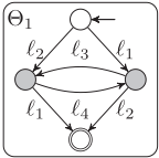
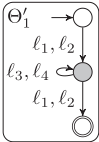
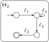
〈0,-1, 0, 2〉 with heuristic value 4, and cost′1 = 〈0, 0, 0, 0〉 and cost′2 = 〈1, 1, 1, 1〉 for F ′ with heuristic value 3.
OCP does not lose information with the stronger restriction to bisimulation shrinking, so the heuristic value is unaffected.
Proposition 6. Let F = 〈Θ1, . . . ,Θn〉 be an FTS and let F ′ = 〈Θ′1 , Θ2, . . . , Θn〉 be the FTS F after shrinking a factor (w.l.o.g. Θ1) with a bisimulation α. Given a solution H, C of OCP(F ) we can construct a solution H′ , C′ of OCP(F ′ ) with at least the same value.
Proof sketch. Instead of H, C, we consider a solution ˆH, C, where ˆHi = Hi for all i ̸= 1 but ˆH1s is the optimal plan cost of s in Θ1 under the costs encoded in C1 for all states s of Θ1. This is the intuitive meaning of the variables H but the LP can admit solutions with lower values. It can be checked that ˆH, C remains a solution and has at least the same value as H, C. For two bisimilar states s ∼ t, we then have ˆH1s = ˆH1t because they have identical plans. We define the desired solution to be like ˆH, C in all components except H′1 , where we set H′1 s = ˆH1s′ for any state s′ mapped to s. As bisimulation shrinking can only combine bisimilar states, H′1 is welldefined. Constraints for goal states and transitions in Θ′1 are validated by the constraints for the goal states and transitions fromΘ1 that induce them.
Note that the proof uses a property that is similar to hpreserving shrinking but the difference is that bisimulation preserves h values under any cost function, in particular under the cost function encoded in C1 , while h-preserving shrinking only considers h-values under the original cost function.
By combining Propositions 5 and 6, we conclude that hOCP is invariant under bisimulation shrinking.
Theorem 4. Let F and F ′ be FTSs such that F ′ results from F with bisimulation shrinking. Then hOCP F = hOCP F ′ .
4.3 Merging
The previous two sections showed transformations that can potentially decrease the value of hOCP . In contrast to these results, we show in this section that the heuristic value of hOCP can only increase after merging.
Proposition 7. Let F = 〈Θ1,Θ2, . . . ,Θn〉 be an FTS and let F ′ = 〈Θm,Θ3, . . . ,Θn〉 be the FTS where two factors (w.l.o.g. Θ1 and Θ2) have been replaced with their synchronized product Θm = Θ1 ⊗ Θ2. Given a solution H, C of OCP(F ), we can construct a solution H′ , C′ of OCP(F ′ ) with the same value.
Proof. We construct the solution as H′m 〈s1,s2〉 = H1s1 + H2s2 and C′m ℓ = C1ℓ + C2ℓ , leaving all other components of H, C
the same. The new solution forms a cost partition for F ′ and has the same objective value. Constraints (1) and (2) for Θm are validated for a goal state or transition by summing the constraints for the goal states or transitions inducing them in the synchronized product.
From Proposition 7 we can conclude that merging can only be beneficial for optimal cost partitioning.
Theorem 5. Let F and F ′ be FTSs such that F ′ results from F with merging two factors. Then hOCP F ≤ hOCP F ′ .
5 Interaction of SCP withM&S
The results on the interaction of OCP and M&S do not allow to draw conclusions for other cost partitioning techniques. In this section, we analyze how applying M&S transformations affects hSCP . To avoid that a difference in the heuristic value is only caused by a different order, we compare compatible orders before and after a M&S transformation.
5.1 Label Reduction
In this section, we consider an FTS F = 〈Θ1, . . . , Θn〉 with labels L and the FTS F ′ = 〈Θ′1 , . . . , Θ′n 〉 with labels L′ that results from applying label reduction λ : L → L′ to F . As all Θ′i in F ′ are derived fromΘi via λ, we compare hSCP before and after label reduction with orders ω and ω′ , where ω′ can be derived from ω by replacing each Θi with Θ′i .
We first show that the value of hSCP can decrease or increase after label reduction. Thereafter, we show that exact label reduction does not affect the value of hSCP .
Theorem 6. Given F , F ′ , ω and ω′ as described above, hSCP F,ω and hSCP F ′ ,ω′ are incomparable.
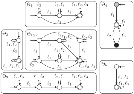
Proof. We provide examples for all three cases. If λ(ℓ) = ℓ for all ℓ ∈ L, we have F = F ′ and ω = ω′ and hence hSCP F,ω = hSCP F ′ ,ω′ . Now consider an FTS F = 〈Θ2,Θ5,Θ3〉 with factors as depicted in Figure 4 and order ω = F. We have hSCP F,ω (sI) = 2. If all labels are mapped to the same label, we get hSCP F ′ ,ω′(sI) = 1, and if only ℓ2 and ℓ3 are mapped to the same label, we get hSCP F ′ ,ω′ (sI ) = 3.
Theorem 7. Given F, F ′ , ω and ω′ as described above. If λ is an exact label reduction, then hSCP F,ω = hSCP F ′ ,ω′ .
Proof sketch. As the label reduction is exact, we know that all combined labels are Θk-combinable. We prove the following statements by an induction over the order ω:
for all 1 ≤ i ≤ n, all states s, all ℓ′ ∈ L′ , and all ℓ ∈ λ-1 (ℓ′ ). The theorem then follows from the first statement. The full proof can be found in a technical report [Sievers et al., 2020b].
5.2 Shrinking
Consider two FTSs F = 〈Θ1, . . .Θn〉 and F ′ = 〈α(Θ1), . . .Θn〉 where w.l.o.g. Θ1 of F is shrunk with abstraction α. The order ω′ for F ′ can be derived from the order ω for F by replacing Θ1 with α(Θ1).
Theorem 8. Given F , F ′ , ω and ω′ as described above, hSCP F,ω and hSCP F ′ ,ω′ are incomparable.
Proof. We provide examples for all three cases. If α = id and hence α(Θ1) = Θ1, we have ω = ω′ and hSCP F,ω = hSCP F ′ ,ω′ . Now consider an FTS F = 〈Θ4, Θ2〉 with factors as depicted in Figure 4 and the order ω = F . We have hSCP F,ω (sI) = 1. If Θ4 is shrunk by combining the black and white states, we get hSCP F ′ ,ω′(sI) = 2, but if Θ4 is shrunk by combining the gray and white states, we get hSCP F ′ ,ω′ (sI ) = 0.
Theorem 9. Given F, F ′ , ω and ω′ as described above. If 〈cost1, . . . , costn〉 is the cost partition computed by hSCP F,ω and α is h-preserving under cost1 then hSCP F,ω = hSCP F ′ ,ω′ .
Proof sketch. Saturated costs in Θi are computed solely with the h-values of states under rci, which are preserved by α for all s ∈ S(α(Θ1)) according to the condition on α.
5.3 Merging
Consider FTS F = 〈Θ1, . . . ,Θn〉 and a merge transformation which w.l.o.g. replaces the factors Θ1 and Θ2 by their product Θ1⊗2 to obtain the FTS F ′ . There are two compatible orders: ω′ replaces Θ1 with Θ1⊗2 and removes Θ2, while ω′′ replaces Θ2 with Θ1⊗2 and removes Θ1.
Theorem 10. Given F, F ′ , ω and ω′ as described above, hSCP F,ω , hSCP F ′ ,ω′ and hSCP F ′ ,ω′′ are incomparable.
Proof. By choosing ω so Θ1 and Θ2 appear consecutively, we have ω′ = ω′′ and it is sufficient to give an example for all three possible cases. If Θ2 is a factor with a single (goal) state s, we have hΘ2 (s, cost2) = 0 and Θ1⊗2 = Θ1 and hence hSCP F,ω = hSCP F ′ ,ω′ .
Now consider an FTS F = 〈Θ1,Θ2,Θ3〉 with factors as depicted in Figure 4 and the order ω = F. We have Algorithm 1 Merge-and-shrink algorithm extended to com-
pute SCP heuristics. Input: FTS F, transformation strategies, size limit, time limit, order strategy Output: Heuristic for F 1: function M&SWITHSCP(F) 2: F ′ ←F 3: H ← ∅ 4: while not TERMINATE(〈F ′ ,Σ, λ〉) do 5: i, j ← MERGESTRATEGY(F ′ ) 6: F ′ ← LABELREDUCTIONSTRATEGY(F ′ ) 7: H ← H ∪ COMPUTESNAPSHOT(F ′ ) 8: Θ′i , Θ′j ← SHRINKSTRATEGY(F ′ , i, j) 9: F ′ ← (F ′ \ {Θi, Θj}) ∪ {Θ′i , Θ′j } 10: F ′ ← (F ′ \ {Θ′i , Θ′j }) ∪ {Θ′i ⊗ Θ′j } 11: end while 12: return maxhSCP∈H hSCP 13: end functionhSCP F,ω (sI) = 3. If Θ1 and Θ2 are merged to Θ1⊗2, we get hSCP F ′ ,ω′(sI) = 2. If we consider an FTS F〈Θ1,Θ2〉 instead, we have hSCP F,ω (sI ) = 1 but hSCP F ′ ,ω′ (sI ) = 2 after merging.
6 Implementation
We now describe our practical approach of integrating label cost partitioning into the M&S algorithm. We focus on SCPs because computing OCPs over large abstractions is often infeasible in practice, but our approach can be used with OCPs in the same way.
Recall that at each step of the M&S algorithm on some FTS F , the factors Θi of the current FTS F ′ induce the factor heuristics hΘi for F . The first and most simple approach simply takes the final factor heuristics of the M&S computation and, instead of computing the maximum over them like hM&S does, combines them into an SCP heuristic (denoted hSCP final ). However, if there is enough time, the M&S algorithm only terminates when there is only one factor left, in which case neither maximizing nor cost partitioning is beneficial.
Therefore, we instead suggest to compute SCP heuristics over the factor heuristics of any intermediate FTS F ′ and to compute the maximum over these SCP heuristics to form the final heuristic. This approach requires to decide when and how often to compute such SCP heuristics. Concerning how often, for simplicity, we decided to take a single snapshot of each ith iteration of M&S. That is, in each ith iteration, we compute a single SCP heuristic over the factor heuristics induced by the current FTS. We experimentally evaluate different values for i. Regarding the choice of when in a given iteration this should be done, our theoretical analysis showed that each transformation can have a positive or negative impact, so we consider computing a snapshot after label reduction, after shrinking, or after merging.
Algorithm 1 shows the M&S algorithm extended to compute SCP heuristics. Compared to regular M&S, it additionally stores the computed SCP heuristics in a set H (line 7). Depending on when to compute the snapshot, line 7 is moved after line 9 (shrinking) or after line 10 (merging). At the end (line 12), instead of computing hM&S over the final F ′ , it computes the maximum heuristic over all SCP heuristics in H, which we denote by hSCP int for this interleaved approach of computing M&S and SCPs. The parameter order strategy specifies in which order to compute SCP heuristics and we explore different choices in the experiments.
A potential drawback of the interleaved approach is that it misses the opportunity to combine factor heuristics of different M&S iterations with extended label cost partitions. We therefore also suggest an offline approach, which, rather than computing an SCP during an iteration, only stores the factor heuristics of that iteration for later use. We exclude factors which have not changed since the last snapshot to avoid duplicates. At the end, we need to use the stored factor heuristics to compute a heuristic. We consider two alternatives: computing a single SCP heuristic, denoted hSCP off , and computing the maximum heuristic over several SCP heuristics computed for diverse orders obtained with the algorithm by Seipp et al. [2020], denoted hSCP off-div . This makes the offline approach more comparable to the interleaved approach that also maximizes over several SCP heuristics. A potential disadvantage of the offline approach is that it needs to store the transition system of each factor heuristic until it computed the SCPs.
Finally, we remark that for all SCP heuristics, we only store useful (non-constant zero) heuristics as suggested by Seipp et al. [2020]. Furthermore, for each factor heuristic used in an SCP, we need to copy the relevant state mapping because further M&S transformations possibly modify it. However, M&S stores state mappings in a tree-like data structure called factored state mappings [Sievers, 2018] which is expensive to copy. Fortunately, only their root node is subject to potential change through M&S transformations. We exploit this by computing shallow copies, reusing subtrees which are guaranteed to not change anymore. We experimentally compare this to the alternative of making full copies.
7 Experiments
We implemented our techniques on top of the M&S implementation of Fast Downward [Helmert, 2006], version 19.12. To evaluate them, we use the following state-of-the-art M&S configuration: shrinking is based on bisimulation and uses a size limit of 50000 on transition systems (allowing exact shrinking also when shrinking is not necessary to respect the size limit); the merge strategy is SCC-DFP [Sievers et al., 2016]; we use exact label reduction; and the main loop is limited to 900s. As benchmarks, we use the tasks of all optimal tracks of all International Planning Competitions, a set consisting of 1827 tasks across 65 domains. Experiments were run on Intel Xeon Silver 4114 CPUs, using Downward Lab [Seipp et al., 2017b]. Each planner run is limited to 1800s and 3.5 GiB. The code, benchmarks, and experimental data are published online [Sievers et al., 2020a].
We use the following order strategies for computing SCPs: random (rnd); creation time of the factors (otn for old to new); the inverse of otn (nto); the greedy orders of Seipp et al. [2020] called maximize heuristic (mh), minimize stolen cost (msc), and maximize heuristic per stolen cost (mhsc). Greedy orders are computed for the initial state.
Number of M&S transformations
| after label reduction | i = 1, shallow | |||||
|---|---|---|---|---|---|---|
| i = 1 i = 2 i = 5 i = 10 | after label r. | 933 | ||||
| full | 922 | 923 | 923 | 916 after | shrinking 933 | |
| shallow | 933 | 930 | 926 | 917 after | merging 925 | |
Table 1: Coverage of hSCP int, rnd computing an SCP every ith iteration after different M&S transformations using shallow or full copies of the factored state mappings.
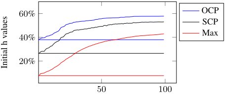
First, we analyze how much better compared to hM&S we can get. Figure 5 reports the development of initial h-values of the factor heuristics after each M&S transformation, when combined with maximization (Max), SCP with a random order, or OCP. In this plot, we only consider the 833 tasks where M&S terminated (including computing the cost partitions). As expected, the combination with cost partitioning dominates the combination with maximization, but SCP is reasonably close to OCP, which justifies its higher practical relevance compared to the more expensive OCP.
Second, we compare hM&S against hSCP final . There are 162 tasks for which M&S computes more than one factor heuristic because it reaches the time limit. Of these tasks, hM&S solves 50 compared to 56 tasks solved by hSCP final regardless of the used order. This is the result we expected: the combination with SCP is usually stronger than the maximization used by hM&S , but since these tasks are the most difficult ones (indicated by M&S reaching the time limit), the difference is small.
Next, we investigate the interleaved SCP approach by varying the parameter i. We also compare full against shallow copies of factored states mappings. The left part of Table 1 shows coverage (number of solved tasks) of hSCP int with a random order (hSCP int, rnd ) when computing snapshots after label reduction. Compared to hM&S , which achieves a coverage of 905, we can see that all variants improve coverage, even when computing a snapshot each iteration (i = 1). While with full copying, there is no visible difference for i = 1, 2, 5, using the memory-efficient shallow copying significantly improves coverage of those variants. For i = 10, performance is similar for full and shallow copies, which can be explained by a lower heuristic quality compared to smaller values of i due to computing fewer SCP heuristics. We use the best configuration i = 1 and shallow copies for the remaining evaluation.
| rnd | otn | nto | mhsc | mh | msc | |
|---|---|---|---|---|---|---|
| hSCP int | 933 | 932 | 928 | 928 | 927 | 930 |
| hSCP off | 841 | 836 | 905 | 869 | 905 | 837 |
| hSCP off-div | 915 | 841 | 904 | 887 | 907 | 838 |
We continue with evaluating when to compute snapshots: after label reduction, shrinking or merging. The right part of Table 1 shows how this affects the coverage of hSCP int, rnd . We observe no difference between the first two choices but a clear benefit over the third. This matches our theoretical results: the value of an SCP heuristic is not affected by exact label reduction and h-preserving shrinking, whereas merging can affect the SCP value arbitrarily. We compute the snapshots after label reduction for the rest of the evaluation.
Finally, we evaluate different order strategies. The first row of Table 2 shows coverage of hSCP int . Somewhat surprisingly, the random order (rnd) performs best. A possible reason is that diversification of orders with interleaved SCPs is obtained through computing SCPs over different factor heuristics in each iteration. Another reason might be that the two basic orders we introduced (otn and nto) as well as the greedy orders by Seipp et al. [2020] (mhsc, mh, msc) are not well suited for our setting.
The latter hypothesis is backed by the evaluation of the offline approach under the same setting as the interleaved approach (i = 1, shallow copies, snapshots after label reduction). The last two rows of Table 2 show coverage of hSCP off and hSCP off-div . Interestingly, even computing a single SCP heuristic (hSCP off ) with orders nto and mh already achieves the same coverage as plain hM&S . Computing diverse orders (hSCP off-div ) strictly improves coverage compared to hSCP off , but only marginally for all order strategies except rnd, which is the best strategy like for the interleaved approach. Compared to hSCP int , hSCP off-div is strictly dominated in terms of total coverage. Again, the most likely explanation is that the order strategies are not strong enough to help the order diversification algorithm to find better orders compared to the diversification implicitly obtained by the interleaved approach.
8 Conclusions
In this paper, we contribute the first combination of cost partitioning with M&S heuristics. Our theoretical analysis investigates the interaction of OCP and SCP with M&S transformations, and our practical implementation significantly improves regular M&S heuristics. In future work, we want to investigate better order strategies for SCPs in the context of M&S and to formalize cost partitioning as a transformation of the M&S framework.
Acknowledgements
We have received funding for this work from the European Research Council (ERC) under the European Union's Horizon 2020 research and innovation programme (grant agreement no. 817639).
@inproceedings{ijcai2020p574,
  title     = {Cost-Partitioned Merge-and-Shrink Heuristics for Optimal Classical Planning},
  author    = {Sievers, Silvan and Pommerening, Florian and Keller, Thomas and Helmert, Malte},
  booktitle = {Proceedings of the Twenty-Ninth International Joint Conference on
               Artificial Intelligence, {IJCAI-20}},
  publisher = {International Joint Conferences on Artificial Intelligence Organization},
  editor    = {Christian Bessiere},
  pages     = {4152--4160},
  year      = {2020},
  month     = {7},
  note      = {Main track},
  doi       = {10.24963/ijcai.2020/574},
  url       = {https://doi.org/10.24963/ijcai.2020/574},
}
TY - CPAPER TI - Cost-Partitioned Merge-and-Shrink Heuristics for Optimal Classical Planning AU - Sievers, Silvan AU - Pommerening, Florian AU - Keller, Thomas AU - Helmert, Malte T2 - Proceedings of the Twenty-Ninth International Joint Conference on Artificial Intelligence, IJCAI-20 PB - International Joint Conferences on Artificial Intelligence Organization PY - 2020 SP - 4152 EP - 4160 DO - 10.24963/ijcai.2020/574 UR - https://doi.org/10.24963/ijcai.2020/574 ER -Copied
Machine-readable versions of this paper, for tools and AI agents:





