
Computing Perfect Heuristics in Polynomial Time: On Bisimulation and Merge-and-Shrink Abstraction in Optimal Planning
Proceedings of the Twenty-Second International Joint Conference on Artificial Intelligence. Pages 1983-1989.
https://doi.org/10.5591/978-1-57735-516-8/IJCAI11-331
© 2011 International Joint Conferences on Artificial Intelligence
Abstract
A* with admissible heuristics is a very successful approach to optimal planning. But how to derive such heuristics automatically? Merge-and-shrink abstraction (M&S) is a general approach to heuristic design whose key advantage is its capability to make very fine-grained choices in defining abstractions. However, little is known about how to actually make these choices. We address this via the well-known notion of bisimulation. When aggregating only bisimilar states, M&S yields a perfect heuristic. Alas, bisimulations are exponentially large even in trivial domains. We show how to apply label reduction — not distinguishing between certain groups of operators — without incurring any information loss, while potentially reducing bisimulation size exponentially. In several benchmark domains, the resulting algorithm computes perfect heuristics in polynomial time. Empirically, we show that approximating variants of this algorithm improve the state of the art in M&S heuristics. In particular, a simple hybrid of two such variants is competitive with the leading heuristic LM-cut.
- [Dräger et al., 2006] Klaus Dräger, Bernd Finkbeiner, and Andreas Podelski. Directed model checking with distance-preserving ab- stractions. In Proc. SPIN 2006, pages 19-34, 2006.
- [Edelkamp, 2001] Stefan Edelkamp. Planning with pattern databases. In Proc. ECP 2001, pages 13-24, 2001.
- [Helmert and Domshlak, 2009] Malte Helmert and Carmel Domsh- lak. Landmarks, critical paths and abstractions: What's the dif- ference anyway? In Proc. ICAPS 2009, pages 162-169, 2009.
- [Helmert and Mattmüller, 2008] Malte Helmert and Robert Mattmüller. Accuracy of admissible heuristic functions in selected planning domains. In Proc. AAAI 2008, pages 938-943, 2008.
- [Helmert et al., 2007] Malte Helmert, Patrik Haslum, and Jörg Hoffmann. Flexible abstraction heuristics for optimal sequential planning. In Proc. ICAPS 2007, pages 176-183, 2007.
- [Helmert, 2006] Malte Helmert. Solving Planning Tasks in Theory and Practice. PhD thesis, University of Freiburg, 2006.
- [Katz and Domshlak, 2009] Michael Katz and Carmel Domshlak. Structural-pattern databases. In Proc. ICAPS 2009, pages 186- 193, 2009.
- [Milner, 1990] Robin Milner. Operational and algebraic semantics of concurrent processes. In Handbook of TCS, pages 1201-1242. 1990.
- [Richter and Helmert, 2009] Silvia Richter and Malte Helmert. Preferred operators and deferred evaluation in satisficing plan- ning. In Proc. ICAPS 2009, pages 273-280, 2009.
References were extracted automatically from the PDF and may contain errors.
Full text extracted automatically from the PDF; figures, tables and equations may differ. The PDF is the version of record.
1 Introduction
Many optimal planning systems are based on state-space search with A∗ and admissible heuristics. The research question is how to derive the heuristic automatically. Merge-andshrink abstraction [Dr¨ager et al., 2006; Helmert et al., 2007], in short M&S, uses solution distance in a smaller, abstract state space to yield a consistent and admissible heuristic.
The abstract state space is built in an incremental fashion, starting with a set of atomic abstractions corresponding to individual variables, then iteratively merging two abstractions - replacing them with their synchronized product - and shrinking them - aggregating pairs of states into one. Thus, despite the exponential size of the state space, M&S allows to select individual pairs of states to aggregate. This freedom in abstraction design comes with significant advantages. M&S dominates most other known frameworks for computing admissible planning heuristics: for any given state, it can with polynomial overhead compute a larger lower bound [Helmert and Domshlak, 2009]. Further, in difference to
Malte Helmert
University of Freiburg Freiburg, Germany helmert@informatik.uni-freiburg.de
most other known frameworks, M&S is able to compute, in polynomial time, perfect heuristics for some benchmark domains where optimal planning is easy [Helmert et al., 2007; Helmert and Mattm¨uller, 2008].
M&S currently does not live up to its promises: (A) in the international planning competition (IPC) benchmarks, it gives worse empirical performance than the currently leading heuristics, in particular LM-cut [Helmert and Domshlak, 2009]; (B) it does not deliver perfect heuristics in the benchmarks where it could. The theoretical power of M&S hinges on the ability to take perfect decisions as to which pairs of states to aggregate. Little is known about how to take such decisions in practice. We herein address this issue, largely solving (B), and making headway towards solving (A).
Our investigation is based on the notion of bisimulation, a well-known criterion under which an abstract state space "exhibits the same observable behavior" as the original state space [Milner, 1990]. Two states s, t are bisimilar if: (1) they agree on whether or not the goal is true; and (2) every transition label, i.e., every planning operator, leads into the same abstract state from both s and t. If we aggregate only bisimilar states during M&S, then the heuristic is guaranteed to be perfect. A coarsest bisimulation can be efficiently constructed, and thus this offers a practical strategy for selecting the states to aggregate. Indeed, this was observed already by Dr¨ager et al. [2006] (in a model checking context). However, bisimulations are exponentially big even in trivial examples, including the aforementioned benchmarks (B). Our key observation is that, for the purpose of computing a heuristic, we can relax bisimulation significantly without losing any information. Namely, we do not need to distinguish the transition labels. Such a fully label-reduced bisimulation still preserves solution distance, while often being exponentially smaller.
Unfortunately, while full label reduction does not affect solution distances per se, its application within the M&S framework is problematic. The merging step, in order to synchronize transitions, needs to know which ones share the same label, i.e., correspond to the same operator. We tackle this by using partial label reductions, ignoring the difference between two labels only if they are equivalent for "the rest" of the M&S construction. We thus obtain, again, a strategy that guarantees to deliver a perfect heuristic. This method largely solves challenge (B), in that its runtime is polynomially bounded in most of the relevant domains.
Even label-reduced bisimulations are often prohibitively big, thus for practicality one needs a strategy to approximate further if required. We experiment with a variety of such strategies, and examine their performance empirically. Each single strategy still is inferior to LM-cut. However, the different strategies exhibit complementary strengths, i.e., they work well in different domains. We thus experiment with simple hybrid planners running two of the stragies sequentially. We find that, addressing challenge (A), one of these hybrids is competitive with LM-cut in the IPC benchmarks, and even outperforms it when ignoring the Miconic domain.
For space reasons, we omit many details and only outline proofs. Full details are available from the authors on request.
2 Background
We consider optimal sequential planning with finite-domain variables. A planning task is a 4-tuple (V,O, s0, s⋆). V is a finite set of variables, where each v ∈ V is associated with a finite domain Dv. A partial state over V is a function s on a subset Vs of V, so that s(v) ∈ Dv for all v ∈ Vs; s is a state if Vs = V. The initial state s0 is a state. The goal s⋆ is a partial state. O is a finite set of operators, each being a pair (pre, eff) of partial states, called its precondition and effect.
The semantics of planning tasks are, as usual, defined via their state spaces, which are (labeled) transition systems. Such a system is a 5-tuple Θ = (S,L, T, s0, S⋆) where S is a finite set of states, L is a finite set of transition labels, T ⊆ S ×L×S is a set of labeled transitions, s0 ∈ S is the start state, and S⋆ ⊆ S is the set of solution states. In the state space of a planning task, S is the set of all states; s0 is identical with the initial state of the task; s ∈ S⋆ if s⋆ ⊆ s; the transition labels L are the operators O; and (s, (pre, eff), s′ ) ∈ T if s complies with pre, s′ (v) = eff(v) for v ∈ Veff, and s′ (v) = s(v) for v ∈ V \ Veff. A plan is a path from s0 to any s⋆ ∈ S⋆. The plan is optimal iff its length is equal to sd(s0), where sd : S → N0 assigns to s the length of a shortest path from s to any s⋆ ∈ S⋆, or sd(s) = ∞ if there is no such path.
A heuristic is a function h : S → N0 ∪{∞}. The heuristic is admissible iff, for every s ∈ S, h(s) ≤ sd(s); it is consistent iff, for every (s, l, s′ ) ∈ T, h(s) ≤ h(s′ ) + 1. As is well known, A∗ with an admissible heuristic returns an optimal solution, and does not need to re-open any nodes if the heuristic is consistent. We will also consider perfect heuristics, that coincide with sd. If we know that h is perfect, then we can extract an optimal plan without any search.
How to automatically compute a heuristic, given a planning task as input? Our approach is based on designing an abstraction. This is a function α mapping S to a set of abstract states Sα. The abstract state space Θα is defined as (Sα, L, T α, sα0 , Sα ⋆ ), where T α := {(α(s), l, α(s′ )) | (s, l, s′ ) ∈ T}, sα0 := α(s0), and Sα ⋆ := {α(s⋆) | s⋆ ∈ S⋆}. The abstraction heuristic hα maps each s ∈ S to the solution distance of α(s) in Θα; hα is admissible and consistent. We will sometimes consider the induced equivalence relation ∼α, defined by setting s ∼α t iff α(s) = α(t).
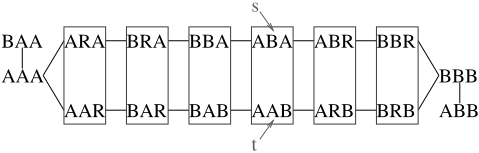
To illustrate abstractions, Figure 1 gives an example. In the Gripper benchmark, one needs to transport n objects from a room A into a room B, with a robot R that can carry two objects at a time. We show here the state space for n = 2, in the simplified situation where the robot can carry only a single object. The planning task has 4 variables, R with DR = {A,B}, F with DF = {0, 1} (hand free?), Oi with DOi = {A,B,R} for i = 1, 2. States in Figure 1 are shown as triples giving the value of R, O1, and O2 in this order (omitting F, whose value is implied). For example, in the state marked "s", the robot is at A, O1 is at B, O2 is at A (and F = 1). The abstraction α is indicated by the (blue) dashed boxes. This abstraction aggregates states - assigns them to the same abstract state - iff they agree on the status of the robot and on the number of objects in each room. Thus the abstraction does not distinguish the upper solution path (transporting O1 first) from the lower one (transporting O2 first). This does not affect solution length, so hα is perfect. The same can be done for arbitrary n, yielding perfect heuristics and polynomial-sized (measured in |Sα|) abstractions.
How to choose a good α in general? Pattern databases (PDBs) [Edelkamp, 2001] simplify this question by limiting α to be a projection. Given V ⊆ V, the projection πV onto V is defined by setting πV (s) to be the restriction of s onto V . πV can be computed very efficiently, and the solution distances in ΘπV can be pre-computed and stored in a table (the PDB) prior to search.
The downside of PDBs is their lack of flexibility in abstraction design. To be computationally efficient, any PDB can consider only a small subset of variables. Thus, even in trivial domains, PDBs cannot compactly represent the perfect heuristic [Helmert et al., 2007]. For example, in Gripper, any polynomial-sized PDB considers only a logarithmic number of objects. The position of the other objects will be abstracted away, thus under-estimating sd to an arbitrarily large extent. For example, in Figure 1, if V = {R, O1}, then s and its right neighbor are aggregated, shortening the upper solution path. Summing over "additive PDBs" does not help, since at most one such PDB may consider the robot position.
Inspired by work in the context of model checking automata networks [Dr¨ager et al., 2006], Helmert et al. [2007] propose M&S abstraction as an alternative allowing more fine-grained abstraction design, selecting individual pairs of states to aggregate. To make such selection feasible in exponentially large state spaces, the approach builds the abstraction in an incremental fashion, iterating between merging and shrinking steps. In detail, an abstraction α is a M&S abstraction over V ⊆ V if it can be constructed using these rules:
- (i) For v ∈ V, π{v} is an M&S abstraction over {v}.
- (ii) If β is an M&S abstraction over V and γ is a function on Sβ , then γ ◦ β is an M&S abstraction over V .
- (iii) If α1 and α2 are M&S abstractions over disjoint sets V1 and V2, then α1 ⊗ α2 is an M&S abstraction over V1 ∪ V2.
It is important to keep these rules in mind since we will be referring back to them throughout the paper. Rule (i) allows to start from atomic projections, i.e., projections π{v} onto a single variable, also written πv in the rest of this paper. Rule (ii), the shrinking step, allows to iteratively aggregate an arbitrary number of state pairs, in abstraction β. Formally, this simply means to apply an additional abstraction γ to the image of β. In rule (iii), the merging step, the merged abstraction α1 ⊗ α2 is defined by (α1 ⊗ α2)(s) := (α1(s), α2(s)). It is easy to see that this definition generalizes PDBs: 1
Proposition 2.1 (Helmert et al., 2007) Let Θ be the state space of a planning task with variables V, and let α be an M&S abstraction over V ⊆ V constructed using only rules (i) and (iii). Then Θα is isomorphic to ΘπV .
Moreover, as Helmert et al. [2007] show, M&S strictly generalizes PDBs in that it can compactly represent the perfect heuristic in domains where PDBs cannot. For example, in Gripper we obtain the perfect heuristic by aggregating states as exemplified in Figure 1.
Proposition 2.1 holds even if we drop the constraint V1 ∩ V2 = ∅ in rule (iii). That constraint plays an important role in the computation of hα. Note that, a priori, this issue is separate from the design of α. We follow Helmert et al. [2007] in that, while designing α, we maintain also the abstract state space Θα (and are thus able to compute hα). In a little more detail, we maintain a transition system Θα, in a way so that Θα is identical with the (mathematically defined) abstract state space Θα of α; note the use of α as a subscript respectively superscript to distinguish these two. The correct maintenance of Θα is trivial for rules (i) and (ii), but is a bit tricky for rule (iii). We need to compute the abstract state space Θα1⊗α2 of α1 ⊗ α2, based on the transition systems Θα1 and Θα2 computed for α1 and α2 beforehand. As an induction hypothesis, assume that Θα1 = Θα1 and Θα2 = Θα2 . We compute Θα1⊗α2 as the synchronized product Θα1 ⊗ Θα2 . This is a standard operation, its state space being Sα1 × Sα2 , with a transition from (s1, s2) to (s′1 , s′2 ) via label l iff (s1, l, s′1 ) ∈ T α1 and (s2, l, s′2 ) ∈ T α2 . For this to be correct, i.e., to have Θα1 ⊗ Θα2 = Θα1⊗α2 , the constraint V1 ∩ V2 = ∅ is required. Namely, this constraint ensures that α1 and α2 are orthogonal in the sense of Helmert et al. [2007], meaning basically that there exists no variable on whose value both abstractions depend. Then:
Theorem 2.2 (Helmert et al., 2007) Let Θ be the state space of a planning task, and let α1 and α2 be orthogonal abstractions of Θ. Then Θα1 ⊗ Θα2 = Θα1⊗α2 .
In practice, we need a merging strategy deciding which abstractions to merge in (iii), and a shrinking strategy deciding which (and how many) states to aggregate in (ii). Helmert et al. do not investigate this in detail. Our main issue herein is with their shrinking strategy. This aggregates states until a size limit N - an input parameter - is reached. The strategy is based exclusively on the initial state and goal distances in the abstract state space at hand; it is f-preserving in that (if possible) it aggregates states only if they agree on these
1 Helmert et al. do not state Proposition 2.1 (or Theorem 2.2 below) in this form, but they follow trivially from their discussion.
v1, . . . , vn := an ordering of V α := πv1 , Θα := Θπv1 /* rule (i) */ σ1 := function projecting operators onto {v2, . . . , vn} apply σ1 to transition labels in Θα for i := 2, . . . , n do α′ := πvi , Θα′ := Θπvi /* rule (i) */ apply σi-1 to transition labels in Θα′ α := α⊗α′ , Θα := Θα ⊗Θα′ /* rule (iii) */ σi := function projecting operators onto {vi+1, . . . , vn} apply σi to transition labels in Θα ∼:= coarsest bisimulation for Θα aggregate all states s, t in α and Θα where s ∼ t /* rule (ii) */endfor
return α and Θα
Figure 2: Overview of M&S-bop algorithm.
distances. This strategy preserves distances locally - in the abstraction at hand - but does not take into account at all the global impact of aggregating states. For example, in a transportation domain, if we consider only the position of a truck, then any states s, t equally distant from the truck's initial and target position can be aggregated: locally, the difference is irrelevant. Globally, however, there are transportable objects to which the difference in truck positions does matter, and thus aggregating s and t results in information loss. Similar situations occur in Gripper, thus the heuristic computed is not perfect although, theoretically, it could be.
3 M&S-bop Overview
Figure 2 outlines our algorithm computing perfect heuristics, M&S-bop (M&S with bisimulation and operator pruning).
The variable ordering v1, . . . , vn will be defined by the merging strategy (a simple heuristic, cf. Section 8). Note that the merging strategy is linear, i.e., α′ is always atomic in the application of rule (iii). Iterating over v1, . . . , vn, the algorithm maintains an abstraction α, along with the transition system Θα, as described earlier. In this way, M&S-bop is a straightforward instance of the M&S framework. Its distinguishing features are (a) the label reduction functions σi that remove operator preconditions/effects pertaining to variables indexed ≤ i, and (b) coarsest bisimulation over the thus label-reduced abstract state spaces. (b) defines the shrinking strategy, which is influenced by (a) because reducing labels changes the bisimulation. Reducing labels may also change the outcome of the synchronized product (rule (iii)), therefore (a) endangers the correctness of Θα relative to Θα.
In the following three sections, we fill in the formal details on (a) and (b), proving (in particular) that the abstraction heuristic hα of α as returned by M&S-bop is perfect, and can be extracted from the returned transition system Θα. We begin by defining bisimulation, and pointing out some basic facts about its behavior in the M&S framework. We then formally define label reduction and the conditions under which it preserves the correctness of Θα. We finally point out that the two techniques can be combined fruitfully.
4 Bisimulation
Bisimulation is a well-known criterion under which abstraction does not significantly change the system behavior. Namely, let Θ = (S, L, T, s0, S⋆) be a transition system. An equivalence relation ∼ on S is a bisimulation for Θ if: (1) s ∼ t implies that either s, t ∈ S⋆ or s, t ̸∈ S⋆; (2) for every pair of states s, t ∈ S so that s ∼ t, and for every transition label l ∈ L, if (s, l, s′ ) ∈ T then there exists t′ s.t. (t, l, t′ ) ∈ T and s′ ∼ t′ . Intuitively, (1) s and t agree on the status of the goal, and (2) whatever operator applies to s applies also to t, leading into equivalent states. An abstraction α is a bisimulation iff the induced equivalence relation ∼α is.
For a comprehensive treatment of bisimulation, see the work by Milner [1990]. There always exists a unique coarsest bisimulation, i.e., a bisimulation that contains all other bisimulations. The coarsest bisimulation can be computed efficiently, in a bottom-up process starting with a single equivalence class containing all states, then iteratively separating non-bisimilar states. This process can be used as a shrinking strategy, and it preserves solution distance at the local level:
Proposition 4.1 Let Θ be a transition system, and let α be a bisimulation for Θ. Then hα is perfect.
This holds because abstract solution paths are real solution paths. Consider some state t, and an abstract solution for t. Say the abstract solution starts with the transition (A, l,A′ ), where A and A′ are abstract states. Since (A, l,A′ ) is a transition in Θα, there exist states s ∈ A and s′ ∈ A′ so that (s, l, s′ ) is a transition in Θ. By construction, we have α(t) = A = α(s) and thus s ∼α t. Thus, by bisimulation property (2), we have a transition (t, l, t′ ) in Θ where s′ ∼α t′ , i.e., α(t′ ) = α(s′ ) = A′ . In other words, there exists a transition from t taking us into the desired state subset A′ . Iterating the argument, we can execute all transitions on the abstract solution for t. The last state t′ reached this way must be a solution state because of bisimulation property (1) and the fact that α(t′ ) is a solution state in Θα.
Note that the argument we just made is much stronger than what is needed to prove that hα is perfect - we preserve the actual solutions, not only their length. That is exactly what we will exploit further below. First, note that Proposition 4.1 tells us nothing about what will happen if we interleave bisimulation with merging steps. This works, too:
Corollary 4.2 Let Θ be the state space of a planning task with variables V. Let α be an M&S abstraction over V ⊆ V constructed so that, in any application of rule (ii), γ is a bisimulation for Θβ . Then α is a bisimulation for ΘπV .
This can be shown by induction over rules (i)-(iii). The claim is obvious for atomic α. Induction over rule (ii) is easy by exploiting a transitivity property of bisimulations. For rule (iii), assume that α1 is a bisimulation for ΘπV1 , and α2 is a bisimulation for ΘπV2 . Since ΘπV1 and ΘπV2 are orthogonal, by Theorem 2.2 their synchronized product is equal to ΘπV1 ⊗πV2 which is isomorphic with ΘπV1∪V2 . We can apply α1 and α2 to the states in ΘπV1∪V2 (applying their component atomic projections to partial states), and it is easy to see that the bisimulation property is preserved. 2
By Corollary 4.2 and Proposition 4.1, if we always stick to bisimulation during step (ii), then we obtain a perfect heuristic. Alas, in practical examples there rarely exist compact bisimulations. For example, in Gripper, the perfect abstraction of Figure 1 is not a bisimulation. If s and t agree on the number of objects in a room, this does not imply that they agree on the operators needed to transport them. For example, s and t as indicated in Figure 1 require to pick up O2 (s) vs. O1 (t). Thus the transition labels into the equivalent states (right neighbors in Figure 1) are different, violating property (2). Indeed, it is easy to see that the size of bisimulations in Gripper is exponential in the number of objects.
2 Dr¨ager et al. [2006] mention a result similar to Corollary 4.2. The result is simpler in their context because, there, the overall state space is defined in terms of the synchronized product operation.
Motivated by the size of bisimulations, Dr¨ager et al. [2006] propose a more approximate shrinking strategy that we will call the DFP shrinking strategy. When building the coarsest bisimulation, the strategy keeps separating states until the size limit N is reached. The latter may happen before a bisimulation is obtained, in which case we may lose information. The strategy prefers to separate states close to the goal, thus attempting to make errors only in more distant states where the errors will hopefully not be as relevant.
The DFP shrinking strategy is not a bad idea; some of the strategies we experiment with herein are variants of it. However, before resorting to approximations, there is a more fundamental issue we can improve. As noted in the proof of Proposition 4.1, bisimulation preserves solution paths exactly. This suits its traditional purpose in model checking. For computing a perfect heuristic, however, it suffices to preserve solution length. In bisimulation property (2), we can completely ignore the transition labels. This makes all the difference in Gripper. States s and t in Figure 1 can reach the same equivalence classes, but using different labels. Ignoring the latter, s and t are bisimilar. Indeed, the perfect abstraction of Figure 1 is such a fully label-reduced bisimulation.
5 Label Reduction
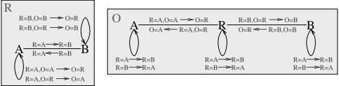
Unfortunately, full label reduction cannot be applied within the M&S framework, at least not without significant information loss during the merging step. Figure 3 shows the atomic projections of our running example from Figure 1. For simplicity, we omit F and show the two variables O1 and O2 in terms of a single generic variable O. Consider the transition label l = ({R = A,O = A}, {O = R}) picking up the object in room A. This transitions O from A to R in ΘπO (right hand side), but does not affect R and hence labels only a self-loop in ΘπR (left hand side). Hence, in the synchronized system ΘπR ⊗ΘπO , as desired the robot does not move while loading the object. If we ignore the difference between l and the label l′ = ({R = A}, {R = B}) moving R, however, then the synchronized systemmay apply l and l′ together, acting as if they were the result of applying the same operator. Thus we may move and pick-up at the same time - a spurious transition not present in the original task.
We now derive a way of reducing subsets of labels during M&S, so that no spurious transitions are introduced, and thus the correctness of Θα relative to Θα is preserved. We remark that a simpler version of the technique, pertaining only to linear merging strategies, was implemented already in the initial version of M&S reported by Helmert et al. [2007]; the technique has not yet been described anywhere.
Let Θ = (S,L, T, s0, S⋆) be a transition system. A label reduction is a function τ mapping L to a label set Lτ . We associate τ with the reduced transition system Θ|τ := (S, Lτ , T|τ , s0, S⋆) where T|τ := {(s, τ(l), s′ ) | (s, l, s′ ) ∈ T}. Labels l1 , l2 ∈ L are equivalent in Θ if, for every pair of states s, s′ ∈ S, (s, l1 , s′ ) ∈ T if and only if (s, l2 , s′ ) ∈ T. We say that τ is conservative for Θ if, for all l1 , l2 ∈ L, τ(l1) = τ(l2) only if l1 and l2 are equivalent. Such label reduction is distributive with the synchronized product:
Lemma 5.1 Let L be a set of labels, let Θ1 and Θ2 be transition systems using L, and let τ be a label reduction on L. If τ is conservative for Θ2 , then Θ1 |τ ⊗Θ2 |τ = (Θ1 ⊗Θ2 )|τ .
For illustration, consider the labels l = ({R = A,O = A}, {O = R}) and l′ = ({R = A}, {R = B}) discussed at the start of this section. These are not equivalent in ΘπO (Figure 3 right), and if τ(l) = τ(l′ ) then, as discussed, ΘπR |τ ⊗ΘπO |τ ̸= (ΘπR ⊗ΘπO )|τ in contrast to Lemma 5.1.
We apply conservative label reduction within M&S by, when considering an abstraction over variable subset V , applying a label reduction conservative for the other variables V \V . A key issue here is that one cannot "reduce in opposite directions". To illustrate, say Θ1 (variables V ) has the single label l1 and Θ2 (variables V \ V ) has the single label l2 ̸= l1 . Then Θ1 ⊗Θ2 contains no transitions at all. However, mapping all labels to some unique symbol r is conservative for each of Θ1 and Θ2 . If we synchronize the systems after this reduction, we obtain a transition between every pair of states.
To avoid said difficulties, we apply label reduction upwards in a sequential ordering of the variables (given by the merging strategy). Let V ⊆ V, and let v1, . . . , vn be an ordering of V . We say that an M&S abstraction α over V allows v1, . . . , vn if α is constructed so that, in any application of rule (iii), there exist i, j, k so that V1 = {vi, . . . , vj} and V2 = {vj+1, . . . , vk}. In other words, the construction of α corresponds to a tree whose leaves are ordered v1, . . . , vn.
Let σn ◦ · · · ◦ σ1 be a chain of label reductions for Θ. We denote τ >i := σi ◦ · · · ◦ σ1 . We say that σn ◦ · · · ◦ σ1 is conservative for v1, . . . , vn if, for each 1 ≤ i < n, τ >i is conservative for each of Θπvi+1 , . . . ,Θπvn . Note that the last reduction σn is not restricted at all, and may thus be a full label reduction mapping all labels to the same unique symbol.
In practice, the label reductions σi we use are those from M&S-bop (cf. Figure 2), projecting operators onto {vi+1, . . . , vn}, i.e., removing any preconditions/effects pertaining to the variables v1, . . . , vi that have already been merged. This chain of label reductions is conservative:
Proposition 5.2 Let Θ be the state space of a planning task with variables V. Let V ⊆ V, and let v1, . . . , vn be an ordering of V . Then operator projection is conservative for v1, . . . , vn, and is maximal among all chained label reductions with this property.
For the first part of the claim, we need τ >i = σi to be conservative - map only equivalent labels (pre, eff), (pre′ , eff′ ) to the same label - for each of Θπvi+1 , . . . ,Θπvn . This holds because (*) (pre, eff) and (pre′ , eff′ ) are equivalent in Θπvj if and only if their projection onto vj is identical. The second part of the claim, maximality, holds in that τ >i maps all equivalent labels to the same label. This follows from the "only if" direction in (*).
Say that in our running example (omitting F) the variable order is R,O1,O2, . . . ,On. Consider again the labels l = ({R = A,O = A}, {O = R}) and l′ = ({R = A}, {R = B}). For i = 1, the robot move l′ is projected onto τ >1 (l′ ) = (∅, ∅), ignoring the information about the robot position. However, τ >1 (l) = ({O = A}, {O = R}), so τ >1 (l) ̸= τ >1 (l′ ) as desired. On the other hand, for i > 1 and every j ≤ i, all labels in ΘπOj will be mapped to (∅, ∅) (compare Figure 3 right), so that the differences between any "already merged" objects will effectively be ignored. For i = n, all labels are mapped to (∅, ∅) so the label reduction is full.
With conservative label reductions, for α that allows v1, . . . , vn, we can maintain Θα during M&S similarly as before. Namely, the label-reduced transition system associated with α, written Θτα, is constructed using these rules:
- (i) If α = πvi for a variable vi ∈ V , then Θτα := Θπvi if i ̸= 1, and Θτα := Θπvi |τ >i if i = 1.
- (ii) If α = γ ◦ β where β is an M&S abstraction and γ is a function on Sβ , then Θτα := (Θτβ )γ .
- (iii) If α = α1 ⊗ α2 where α1 (α2) is an M&S abstraction of Θ over V1 = {vi, . . . , vj} (V2 = {vj+1, . . . , vk}), then Θτα := Θτα1 ⊗Θτα2 if i ̸= 1, and Θτα := (Θτα1 ⊗ Θτα2 |τ >j )|σk ◦···◦σj+1 if i = 1.
In words, we apply label reduction only if the underlying variable set V starts at the first variable v1, and we choose the reduction pertaining to the last variable in V . This construction is correct relative to Θα, in the following sense:
Theorem 5.3 Let Θ be the state space of a planning task with variables V. Let V ⊆ V, and let v1, . . . , vn be an ordering of V . Let σn ◦ · · · ◦σ1 be a chained label reduction for Θ that is conservative for v1, . . . , vn, and let α be an M&S abstraction over V that allows v1, . . . , vn. Then Θτα = Θα|τ >n .
Note here that "the correctness of Θα relative to Θα" is now interpreted in a different way. The transition system Θτα we maintain is no longer equal to the abstract state space Θα, but instead to the label-reduced version Θα|τ >n of that abstract state space. Since, obviously, the labels are irrelevant for hα, the heuristic computed is the same.
The proof of Theorem 5.3 is a bit technical, but essentially simple. We prove by induction over the construction of α that, for any intermediate abstraction β over {vi, . . . , vj}, Θτβ = Θβ if i ̸= 1, and Θτβ = Θβ |τ >j if i = 1. The key step is induction over rule (iii) when i = 1. Since τ >j is conservative for each of Θπvj+1 , . . . , Θπvk , we can easily conclude that τ >j is conservative for Θτα2 . The claim then follows by applying Lemma 5.1 and Theorem 2.2.
Summing up, whenever during M&S we face an abstraction over variables v1, . . . , vj, we can project the operators labeling the transitions onto the remaining variables vj+1, . . . , vn. We then still obtain the correct (label-reduced) abstract state space. In the initial implementation of Helmert et al. [2007], the motivation for doing so was the reduced number of labels - planning tasks often contain many operators, so this was time- and space-critical. Here, we observe that label reduction favorably interacts with bisimulation.
6 Bisimulation and Label Reduction
Label reduction obviously preserves Proposition 4.1:
Proposition 6.1 Let Θ be a transition system, τ be a label reduction, and α a bisimulation for Θ|τ . Then hα is perfect.
Proposition 6.1 is important because, as shown by our running example, label reduction may make a big difference:
Proposition 6.2 There exist families F of transition systems Θ with associated label reductions τ so that the coarsest bisimulation for Θ|τ is exponentially smaller than the coarsest bisimulation for Θ.
Corollary 4.2 tells us that, if the shrinking strategy sticks to bisimulation of the original (non label-reduced) abstract state spaces, then the final outcome will be a bisimulation. Does a similar result hold if we stick to bisimulation of the label-reduced abstract state spaces? Unsurprisingly, the answer is "yes". Given variables v1, . . . , vn and a chained label reduction σn ◦· · ·◦σ1 , we say that α is constructed by labelreduced bisimulation if it is constructed so that, in any application of rule (ii) where β is over the variables {vi, . . . , vj}: if i ̸= 1 then γ is a bisimulation for Θβ ; if i = 1 then γ is a bisimulation for Θβ |τ >j . By combining the proofs of Corollary 4.2 and Theorem 5.3, we get:
Theorem 6.3 Let Θ be the state space of a planning task with variables V. Let V ⊆ V, and let v1, . . . , vn be an ordering of V . Let σn ◦ · · · ◦ σ1 be a chained label reduction for Θ that is conservative for v1, . . . , vn, and let α be an M&S abstraction constructed by label-reduced bisimulation. Then α is a bisimulation for ΘπV |τ >n.
By Theorem 6.3 and Proposition 6.1, if α is constructed by label-reduced bisimulation, then hα is perfect. With Proposition 5.2, this hold for α as returned by M&S-bop. By Theorem 5.3 we can maintain the suitable abstract state spaces. In particular, hα can be extracted from M&S-bop's returned transition system Θα. We will see next that M&S-bop has polynomial runtime in quite a number of benchmarks.
7 Domain-Specific Performance Bounds
We measure the performance of M&S-bop in terms of bounds on abstraction size, i.e., the number of abstract states. Runtime is a polynomial function of abstraction size. We express the bounds as functions of domain parameters like the number of objects. Polynomial bounds on abstraction size are possible only in domains with polynomial-time optimal solution algorithms. Helmert [2006] identifies six such domains in the IPC benchmarks: Gripper, Movie, PSR, Schedule, and two variants of Promela. Helmert et al. [2007] state that for each of these except PSR there exist suitable merging and shrinking strategies, but do not provide a way to come up with such strategies automatically. We begin with an easy result:
Proposition 7.1 Let P = {Πn} be the family of Gripper respectively Ext-Movie planning tasks, where n is the number of objects respectively snacks. Then, for any merging strategy, abstraction size for M&S-bop in P is bounded by a cubic respectively linear function in n.
Ext-Movie is an extended version of Movie, allowing to scale the number of snacks. Both results hold because the M&S-bop shrinking strategy aggregates states that agree on the relevant object counts (number of objects in a room, number of snacks already obtained). It should be noted that label reduction is really needed here - in both domains, non-labelreduced bisimulations are exponentially large. The same holds true for all domains discussed below.
We next consider scheduling-like domains, where each task consists of some machines used to change the features f(o) of processable objects o. The relevant property is that, for o ̸= o′ , f(o) and f(o′ ) are mutually independent, i.e., not affected by any common operator - processing an object may affect the status of the machines but does not have immediate consequences for any other object. It is easy to see that the STRIPS variant Schedule-Strips of IPC'00 Schedule is a scheduling-like domain. We thus have:
Proposition 7.2 Let P = {Πn} be the family of ScheduleStrips planning tasks, where n is the number of processable objects. There exists a merging strategy so that abstraction size for M&S-bop in P is bounded by a polynomial in n.
For Promela, this investigation is difficult because M&Sbop depends directly on task syntax, and the IPC'04 Promela domains are syntactically very complicated (compiled from Promela into an expressive PDDL dialect). For a straightforward direct encoding of one of the domains (Dining Philosophers), we found that M&S-bop exhibits exponential behavior. However, a variant that we tentatively named greedy bisimulation gives a polynomial bound. Greedy bisimulation demands bisimulation property (2) only for transitions (s, l, s′ ) where sd(s′ ) ≤ sd(s). Under certain additional conditions on the planning task - which hold in Dining Philosophers - greedy bisimulation results in a perfect heuristic.
Of course, M&S-bop is not omnipotent. For example, say we extend Gripper by scaling the number of robot hands. Then, for any merging strategy, there exists a shrinking strategy so that abstraction size is polynomially bounded. However, M&S-bop does not have such a bound. Robot hands H appear as object-variable values ("O = H") in the effect of pick-up operators. So, unless all object variables were already merged, operator projection does not remove these distinctions, and states using different hands are not bisimilar.
8 Experiments
In most benchmark domains, coarsest bisimulations are still large even under operator projection. We thus designed a family of (mostly) more approximate shrinking strategies. The family is characterized by 3 parameters: (1) overall scheme, (2) bisimulation variant, (3) label reduction on/off. For (1), the options are DFP shrinking strategy with abstraction size limit N vs. coarsest bisimulation without size limit. The former will be indicated by "DFP" in the strategy's name, the latter will be indicated by "M&S-". For (2), the options are bisimulation vs. greedy bisimulation. The strategy name is extended with "b" respectively "g". In (3), we do vs. do not use operator projection. If we do, "op" is attached to the name. In the DFP-g options, we use greedy bisimulation only if bisimulation would break the size limit. Our merging strategy is linear, and follows Fast-Downward's "level heuristic". This orders variables "closest to the root of the causal graph" up front, so that, in operator projection, the most influential variables are projected away earlier on.
| Domain | Hybrid | LM-cut | SP | DFP-b | N=10K DFP-bop | DFP-gop | HHH | DFP-b | N=100K DFP-bop | DFP-gop | HHH | DFP-b | N=200K DFP-bop | DFP-gop | HHH | No bound M&S-b | on M&S-bop | N M&S-gop |
|---|---|---|---|---|---|---|---|---|---|---|---|---|---|---|---|---|---|---|
| airport | 22 | 28 | 21 | 23 | 23 | 23 | 19 | 15 | 15 | 15 | 13 | 11 | 11 | 11 | 12 | 1 | 1 | 22 |
| blocks | 21 | 28 | 21 | 21 | 21 | 21 | 18 | 18 | 18 | 18 | 19 | 18 | 18 | 18 | 19 | 6 | 6 | 21 |
| depots | 7 | 7 | 7 | 7 | 7 | 7 | 7 | 7 | 7 | 7 | 3 | 5 | 6 | 6 | 3 | 1 | 1 | 7 |
| driverlog | 13 | 13 | 13 | 12 | 13 | 13 | 12 | 12 | 12 | 13 | 13 | 12 | 12 | 13 | 14 | 4 | 5 | 12 |
| freecell | 16 | 15 16 | 15 | 16 | 16 | 15 | 4 | 6 | 6 | 9 | 4 | 3 | 3 | 6 | 3 | 3 | 16 | |
| grid | 3 | 2 | 1 | 1 | 2 | 2 | 2 | 1 | 3 | 3 | 2 | 0 | 3 | 3 | 0 | 0 | 0 | 2 |
| gripper | 20 | 7 | 7 | 7 | 11 | 11 | 7 | 7 | 20 | 20 | 7 | 7 | 20 | 20 | 7 | 6 | 20 | 7 |
| logistics00 | 20 | 20 | 22 | 20 | 20 | 20 | 16 | 20 | 20 | 20 | 21 | 20 | 20 | 20 | 22 | 10 | 10 | 16 |
| logistics98 | 5 | 6 | 6 | 4 | 4 | 4 | 5 | 5 | 5 | 5 | 5 | 5 | 5 | 5 | 5 | 2 | 1 | 4 |
| miconic | 67 | 141 | 53 | 55 | 56 | 56 | 55 | 55 | 65 | 65 | 55 | 55 | 67 | 67 | 56 | 40 | 56 | 50 |
| mprime | 23 | 22 | 23 | 18 | 19 | 19 | 21 | 8 | 12 | 12 | 14 | 4 | 9 | 9 | 9 | 1 | 1 | 23 |
| mystery | 15 | 16 | 15 | 13 | 13 | 13 | 14 | 7 | 8 | 8 | 11 | 6 | 6 | 6 | 7 | 2 | 3 | 15 |
| openstacks | 7 | 7 | 7 | 7 | 7 | 7 | 7 | 7 | 7 | 7 | 7 | 7 | 7 | 7 | 7 | 7 | 7 | 7 |
| pathways | 4 | 5 | 4 | 4 | 4 | 4 | 4 | 4 | 4 | 4 | 4 | 4 | 4 | 4 | 4 | 4 | 4 | 4 |
| pipesworld-notank | 15 | 17 | 14 | 15 | 17 | 17 | 9 | 9 | 9 | 9 | 2 | 6 | 6 | 6 | 0 | 2 | 2 | 15 |
| pipesworld-tank | 16 | 11 | 10 | 13 | 14 | 14 | 13 | 7 | 8 | 8 | 7 | 4 | 7 | 7 | 5 | 2 | 2 | 16 |
| psr | 50 | 49 | 49 | 49 | 49 | 49 | 50 | 49 | 49 | 49 | 50 | 49 | 49 | 50 | 50 | 43 | 45 | 50 |
| rovers | 8 | 7 | 6 | 6 | 7 | 7 | 7 | 7 | 8 | 8 | 7 | 6 | 8 | 8 | 7 | 4 | 4 | 6 |
| satellite | 7 | 7 | 6 | 6 | 6 | 6 | 6 | 6 | 7 | 7 | 6 | 6 | 7 | 7 | 6 | 4 | 6 | 6 |
| tpp | 7 | 6 | 6 | 6 | 6 | 6 | 6 | 6 | 7 | 7 | 6 | 6 | 7 | 7 | 6 | 5 | 5 | 6 |
| trucks | 7 | 10 | 7 | 6 | 7 | 7 | 6 | 5 | 7 | 7 | 6 | 5 | 7 | 7 | 6 | 4 | 4 | 6 |
| zenotravel | 11 | 13 | 11 | 9 | 11 | 11 | 11 | 9 | 12 | 12 | 11 | 8 | 11 | 11 | 11 | 5 | 6 | 9 |
| Total | 364 | 437 | 325 | 317 | 333 | 333 | 310 | 268 | 309 | 310 | 278 | 248 | 293 | 295 | 262 | 156 | 192 | 320 |
| 272 | 228 | 136 | 270 | |||||||||||||||
| w/o miconic | 297 | 296 | 262 | 277 | 277 | 255 | 213 | 244 | 245 | 223 | 193 | 226 | 206 | 116 | ||||
| Total M&S built | 621 | 736 | 735 | 699 | 368 | 518 | 518 | 493 | 321 | 461 | 458 | 441 | 156 | 192 | 802 |
We experiment with: the previous M&S heuristic HHH [Helmert et al., 2007]; LM-cut [Helmert and Domshlak, 2009], the currently leading heuristic for optimal planning; and structural patterns (SP) [Katz and Domshlak, 2009], a competitive heuristic related to ours in that it is based on (implicit) abstract state spaces. Our implementation is on top of Fast-Downward, with the same A∗ implementation for all heuristics. We ran all IPC benchmarks supported by LMcut and HHH. The experiments were performed on dual-CPU Opteron 2384 machines, running eight experiments simultaneously in order to fully utilize the available (eight-core) machines. Each planner instance ran on a single core with a time limit of 30 minutes and a memory limit of 2 GB.
Different shrinking strategies sometimes result in complementary strengths (better performance in different domains). Thus we experimented also with all hybrid planners running any two of these strategies, sequentially with a 15 minute limit for each. The best, in terms of total coverage, of these 2-option combinations runs M&S-gop, and DFP-gop with N=200K. This is simply called "Hybrid" in what follows.
Table 1 gives the coverage data. Consider first the "no bound on N" columns on the right hand side. Comparing M&S-b with M&S-bop, we see that operator projection improves performance significantly. Recall that the heuristic in both cases is guaranteed to be perfect, so no actual search is needed in the 192 tasks where M&S-bop succeeds. The effect of using greedy bisimulation (which in general forfeits this guarantee) is dramatic. Note in particular that the number of instances where the abstraction can be built completely - without any size bound - goes up to 802. Interestingly, the effect of the parameter changes is reversed when using DFP: there, operator projection has a much larger impact on performance than greedy bisimulation.
DFP-bop dominates DFP-b (solves at least as many tasks) in 65 of the 66 combinations of domain and N value. DFPgop dominates HHH in the total, and in 50 of these combinations; Hybrid dominates HHH in 64 combinations. SP is more competitive, but is inferior in the total to Hybrid as well as to DFP-bop and DFP-gop with N = 10K. LMcut clearly dominates the total, but this is largely due to Miconic-STRIPS, where LM-cut delivers an exceptionally high-quality heuristic. Disregarding this domain, Hybrid solves 1 more task than LM-cut. In 11 of the 22 domains, Hybrid is one of the top performers, and in 4 more domains, only one task separates it from the top performer.
Coverage is a function of the trade-off between the quality of a heuristic, and the effort needed for computing it. Due to the multitude of domains and algorithms tested, it is beyond the scope of this paper to give detailed data. We provide a summary using Richter and Helmert [2009]'s expansions score (E) and total-runtime score (T). Both range between 0 and 100, for each individual instance. E = 100 if ≤ 100 expansions were made, E = 0 if ≥ 1, 000, 000 expansions were made. In between, E interpolates logarithmically, so that an additive difference of 7.53 in scores corresponds to a factor 2. Similarly, T = 100 for runtimes ≤ 1 second, T = 0 for time-outs, and doubling the runtime decreases the score by about 9.25. The advantage of these scores is that they are absolute, i.e., there is no need to restrict the set of instances considered to those solved by all planners. 3
3 Experimenting with such summaries, we found that they often misrepresented the results. For example, on instances solved by both, M&S-gop beats LM-cut even in some domains where LM-cut
| X = DFP-bop | = HHH | |||||||||||||
|---|---|---|---|---|---|---|---|---|---|---|---|---|---|---|
| Y D | =DFP-b E | Y =DFP-gop T D | Y E T D | =M&S-gop E | Y T D | X =DFP-gop E | Y T D | =M&S-gop E | T | Y D | X =DFP-gop E | = LM-cut Y T D | =M&S-gop E | T |
| blocks mystery log98 log00 psr airport rovers depots trucks freecell tpp driverlog miconic mprime grid satellite gripper | 3.7 0.4 | -1.7 driverlog 5.2 mystery | 1.2 mystery | 9.2 | 33.6 gripper | 40.6 | 25.7 pipesnota | 10.2 | 48.2 | gripper | 41.9 | 30.2 freecell | 0.5 | 33.6 |
| 1.9 1.2 -0.2 blocks | 7.9 | 5.5 satellite | 23.7 | 8.8 blocks | 8.6 | 14.7 | openstack | 21.9 | 9.7 gripper | -0.7 | 5.3 | |||
| -0.6 | 0.1 psr | 0.8 0.2 depots | 1.6 | 10.4 pipesnota | 21.7 | 28.1 mystery | 3.5 | 27.0 | pipesnota | 8.1 | 14.6 psr | -1.1 | 4.5 | |
| openstack | -0.8 | -0.4 rovers | 0.5 0.7 mprime | 1.1 | 38.2 pathways | 13.7 | 3.9 airport | 2.2 | 21.5 | freecell | 4.1 | 5.9 pipesnota | -2.1 | 36.4 |
| -0.9 | -0.9 freecell | 0.4 psr | -2.0 | 3.0 pipestank | 9.3 | 21.5 depots | 1.6 | 14.1 | log00 | 3.6 | 2.7 openstack | -6.6 | 11.5 | |
| -1.0 | 0.9 log98 | 0.5 0.4 0.7 freecell | -3.1 | airport | 8.4 | 0.0 freecell | -0.5 | 27.0 | satellite | 2.4 | -5.8 blocks | -14.0 | -10.1 | |
| -1.0 | -0.7 satellite | 0.3 -0.5 airport | -6.2 | 28.1 22.2 grid | 7.3 | 10.3 pipestank | -0.7 | 43.2 | psr | 1.6 | 1.7 tpp | -15.3 | -4.5 | |
| -1.3 | -5.4 pipestank | 0.3 -0.8 log98 | -8.4 | -5.6 miconic | 6.1 | 2.0 mprime | -1.0 | 27.7 | tpp | -2.2 | -9.4 pipestank | -17.0 | 3.7 | |
| -1.6 | 0.1 pipesnota | 0.2 -0.1 driverlog | -9.0 | 4.2 zenotravel | 4.9 | 3.0 gripper | -2.0 | 0.8 | pipestank | -5.6 | -16.3 depots | -19.8 | 14.9 | |
| -4.1 | -4.9 tpp | 0.1 0.5 rovers | -9.5 | -7.3 trucks | 3.4 | 4.5 grid | -3.8 | 5.8 | driverlog | -9.3 | -1.8 driverlog | -20.3 | 1.2 | |
| -4.2 | 3.7 trucks | 0.1 -0.1 pipestank | -10.0 | 21.7 freecell | 3.1 | -0.6 trucks | -6.8 | 0.1 | grid | -9.5 | 9.9 grid | -20.6 | 5.4 | |
| -4.4 | -1.9 log00 | 0.1 -0.2 trucks | -10.1 | -4.5 rovers | 1.1 | 1.9 zenotravel | -6.9 | -6.4 | rovers | -13.5 | -7.7 mystery | -21.5 | 2.5 | |
| zenotravel | -6.8 | -13.9 zenotravel | 0.1 -0.5 grid | -11.1 | -4.0 blocks | 0.2 | 8.7 miconic | -7.2 | -3.1 | zenotravel | -15.6 | -1.8 mprime | -23.1 | 9.0 |
| -6.9 | -2.4 airport | 0.0 0.7 pipesnota | -11.2 | 19.2 openstack | 0.1 | 1.4 rovers | -8.9 | -6.2 | pathways | -15.8 | -16.1 rovers | -23.5 | -15.8 | |
| -7.7 | -2.2 grid | 0.0 0.6 zenotravel | -11.6 | -9.9 depots | -0.3 | 4.1 pathways | -12.4 | 8.8 | depots | -21.7 | 4.8 log00 | -24.9 | -9.5 | |
| pipestank | -7.9 | -2.3 miconic | 0.0 0.1 tpp | -12.9 | -3.5 tpp | -0.4 | -0.1 psr | -13.0 | 0.6 | blocks | -22.4 | -16.1 zenotravel | -27.4 | -11.2 |
| pipesnota | -9.4 | 2.9 gripper | 0.0 0.0 miconic | -13.4 | -5.0 mprime | -2.1 | -10.6 log98 | -13.3 | -8.8 | mprime | -24.2 | -29.3 satellite | -38.9 -16.5 | |
| -10.4 | 0.2 mprime | 0.0 -0.1 log00 | -21.1 | -12.5 driverlog | -4.4 | -3.6 tpp | -13.4 | -4.2 | mystery | -29.5 | -31.3 airport | -39.2 -15.3 | ||
| pathways | -11.0 | -1.7 openstack | 0.0 -0.1 pathways | -26.1 | 4.7 mystery | -4.5 | -6.9 driverlog | -15.4 | -0.6 | trucks | -31.9 | -20.6 pathways | -41.9 -11.2 | |
| -11.2 | -23.8 pathways | 0.0 -0.1 openstack | -28.5 | 1.8 log98 | -4.9 | -3.4 satellite | -17.5 | -1.9 | airport | -33.0 | -36.8 trucks | -42.1 -25.0 | ||
| -28.1 | -10.5 depots | -0.3 0.4 satellite | -41.0 | -11.2 log00 | -6.8 | 4.2 log00 | -28.1 | -8.1 | log98 | -47.5 | -24.4 log98 | -55.9 | -29.8 | |
| -37.6 | -25.7 blocks | -0.5 -0.5 gripper | -42.6 | -24.9 psr | -10.3 | 2.2 openstack | -28.5 | 2.1 | miconic | -66.5 | -56.8 miconic | -80.0 | -61.9 | |
| Total | -6.9 | -3.6 Total | 0.3 0.1 Total | -11.7 | 4.8 Total | 5.0 | 4.6 Total | -7.0 | 9.3 | Total | -12.4 | -8.4 Total | -24.3 | -3.8 |
Table 2 considers 7 pairs of heuristics X, Y . The 3 pairs in the left part illustrate the differences between the shrinking strategies proposed herein. We do not include M&S-b and M&S-bop because their expansions behavior is not interesting: they either have perfect expansions, or fail. Comparing X = DFP-bop to Y = DFP-b, we clearly see the advantage of operator projection. E(Y ) - E(X) is negative for 20 of 22 domains, meaning that X has fewer expansions. The picture is not quite as clear for runtime because DFP-bop sometimes generates more overhead (taking more time to reach the size limit N). Comparing X = DFP-bop to Y = DFP-gop, we clearly see that the performance difference is very small. By contrast, X = DFP-bop vs. Y = M&S-gop exhibits a huge variance, showing their complementary strengths. This reflects the fact that these two strategies are quite different. M&S-gop enforces bisimulation only on "sd(s′ ) ≤ sd(s)" transitions, but on all of those; DFP-variants enforce bisimulation everywhere but drop it completely if N is exceeded. The former has the edge in heuristic quality (E(Y )-E(X) is negative for 18 domains), the latter is better in total runtime since building the abstraction generates less overhead (e.g., consider the pipesworld-notankage domain).
The middle and right parts of Table 2 show the competition with HHH respectively LM-cut. DFP-gop clearly beats HHH in expansions, and it largely keeps this advantage in runtime. M&S-gop most often produces worse heuristics than HHH, but with less overhead and thus better runtime. As for LM-cut, without any doubt this remains the most informative heuristic here - only in a few domains does DFP-gop manage to beat it. Everywhere else, the question is whether the faster heuristic calls for M&S (amortizing the cost for creating the abstraction in the first place) make up for the larger search space. For DFP-gop, this is the case only in depots. For M&S-gop, this happens in 11 of the domains, and partly to a considerable extent (e.g. freecell, blocks, depots, mprime).
actually scales better - because M&S-gop's cheap heuristic solves the small tasks very quickly, and times out on the larger ones.
9 FutureWork
Our immediate future work concerns greedy bisimulation. First results suggest that there are many other interesting bisimulation variants along these lines, and corresponding conditions under which they yield perfect heuristics. The guiding idea is to test conditions on the degree and form of interactions between the current variable and the remaining ones, using the outcome to fine-tune the subset of transitions for which bisimulation property (2) is demanded.
@inproceedings{ijcai2011p331,
  title     = {Computing Perfect Heuristics in Polynomial Time: On Bisimulation and Merge-and-Shrink Abstraction in Optimal Planning},
  author    = {Nissim, Raz and Hoffmann, Jörg and Helmert, Malte},
  booktitle = {Proceedings of the Twenty-Second International Joint Conference on
               Artificial Intelligence, {IJCAI-11}},
  publisher = {AAAI Press/International Joint Conferences on Artificial Intelligence},
  editor    = {Toby Walsh},
  pages     = {1983--1989},
  year      = {2011},
  month     = {7},
  doi       = {10.5591/978-1-57735-516-8/IJCAI11-331},
  url       = {https://doi.org/10.5591/978-1-57735-516-8/IJCAI11-331},
}
TY - CPAPER TI - Computing Perfect Heuristics in Polynomial Time: On Bisimulation and Merge-and-Shrink Abstraction in Optimal Planning AU - Nissim, Raz AU - Hoffmann, Jörg AU - Helmert, Malte T2 - Proceedings of the Twenty-Second International Joint Conference on Artificial Intelligence, IJCAI-11 PB - AAAI Press/International Joint Conferences on Artificial Intelligence PY - 2011 SP - 1983 EP - 1989 DO - 10.5591/978-1-57735-516-8/IJCAI11-331 UR - https://doi.org/10.5591/978-1-57735-516-8/IJCAI11-331 ER -Copied
Machine-readable versions of this paper, for tools and AI agents:





