
An Attention-based Model for Conversion Rate Prediction with Delayed Feedback via Post-click Calibration
Proceedings of the Twenty-Ninth International Joint Conference on Artificial Intelligence. Main track. Pages 3522-3528.
https://doi.org/10.24963/ijcai.2020/487
Keywords
- Humans and AI: Personalization and User Modeling
- Multidisciplinary Topics and Applications: Information Retrieval
Abstract
Conversion rate (CVR) prediction is becoming increasingly important in the multi-billion dollar online display advertising industry. It has two major challenges: firstly, the scarce user history data is very complicated and non-linear; secondly, the time delay between the clicks and the corresponding conversions can be very large, e.g., ranging from seconds to weeks. Existing models usually suffer from such scarce and delayed conversion behaviors. In this paper, we propose a novel deep learning framework to tackle the two challenges. Specifically, we extract the pre-trained embedding from impressions/clicks to assist in conversion models and propose an inner/self-attention mechanism to capture the fine-grained personalized product purchase interests from the sequential click data. Besides, to overcome the time-delay issue, we calibrate the delay model by learning dynamic hazard function with the abundant post-click data more in line with the real distribution. Empirical experiments with real-world user behavior data prove the effectiveness of the proposed method.
- [Abadi et al., 2016] Martín Abadi, Paul Barham, Jianmin Chen, Zhifeng Chen, Andy Davis, Jeffrey Dean, Matthieu Devin, Sanjay Ghemawat, Geoffrey Irving, Michael Isard, Manjunath Kudlur, Josh Levenberg, Rajat Monga, Sherry Moore, Derek Gordon Murray, Benoit Steiner, Paul A. Tucker, Vijay Vasudevan, Pete Warden, Martin Wicke, Yuan Yu, and Xiaoqiang Zheng. Tensorflow: A system for large-scale machine learning. In OSDI, pages 265-283. USENIX Association, 2016.
- [Bahdanau et al., 2014] Dzmitry Bahdanau, Kyunghyun Cho, and Yoshua Bengio. Neural machine translation by jointly learning to align and translate. Computer Science, 2014.
- [Chapelle, 2014] Olivier Chapelle. Modeling delayed feed- back in display advertising. In KDD, pages 1097-1105, 2014.
- [Cho et al., 2014] Kyunghyun Cho, Bart Van Merrienboer, Caglar Gulcehre, Dzmitry Bahdanau, Fethi Bougares, Holger Schwenk, and Yoshua Bengio. Learning phrase representations using rnn encoder-decoder for statistical machine translation. Computer Science, 2014.
- [Fawcett, 2005] Tom Fawcett. An introduction to roc analy- sis. Pattern Recognition Letters, 27(8):861-874, 2005.
- [Ji et al., 2017] Wendi Ji, Xiaoling Wang, and Feida Zhu. Time-aware conversion prediction. Frontiers Comput. Sci., 11(4):702-716, 2017.
- [Karatzoglou et al., 2016] Alexandros Karatzoglou, Balázs Hidasi, Domonkos Tikk, Oren Sar Shalom, Haggai Roit- man, Bracha Shapira, and Lior Rokach, editors. RecSys. ACM, 2016.
- [Lee et al., 2012] Kuang-chih Lee, Burkay Orten, Ali Das- dan, and Wentong Li. Estimating conversion rate in dis- play advertising from past erformance data. In KDD, pages 768-776, 2012.
- [Lin and Wong, 1990] J Lin and SKM Wong. A new directed divergence measure and its characterization. International Journal Of General System, 17(1):73-81, 1990.
- [Lu et al., 2017] Quan Lu, Shengjun Pan, Liang Wang, Jun- wei Pan, Fengdan Wan, and Hongxia Yang. A practical framework of conversion rate prediction for online display advertising. In ADKDD, pages 9:1-9:9, 2017.
- [Miller Jr, 2011] Rupert G Miller Jr. Survival analysis, vol- ume 66. John Wiley & Sons, 2011.
- [Rosales et al., 2012] Rómer Rosales, Haibin Cheng, and Eren Manavoglu. Post-click conversion modeling and analysis for non-guaranteed delivery display advertising. In WSDM, pages 293-302. ACM, 2012.
- [Safari et al., 2017] Abdollah Safari, Mac Kay Altman, and Thomas M. Loughin. Display advertising: Estimating con- version probability efficiently. 2017.
- [Wang et al., 2017] Y. Wang, J. Xu, A. Wu, M. Li, Y. He, J. Hu, and W. P. Yan. Telepath: Understanding users from a human vision perspective in large-scale recommender systems. 2017.
- [Xiao et al., 2018] Ma Xiao, Liqin Zhao, Huang Guan, Wang Zhi, Zelin Hu, Xiaoqiang Zhu, and Kun Gai. En- tire space multi-task model: An effective approach for es- timating post-click conversion rate. 2018.
- [Yan et al., 2014] Ling Yan, Wu-Jun Li, Gui-Rong Xue, and Dingyi Han. Coupled group lasso for web-scale CTR pre- diction in display advertising. In Proceedings of the 31th International Conference on Machine Learning, ICML 2014, Beijing, China, 21-26 June 2014, pages 802-810, 2014.
- [Yang et al., 2016] Hongxia Yang, Quan Lu, Angus Xianen Qiu, and Chun Han. Large scale CVR prediction through dynamic transfer learning of global and local features. In Proceedings of the 5th International Workshop on Big Data, Streams and Heterogeneous Source Mining: Algo- rithms, Systems, Programming Models and Applications, BigMine 2016, pages 103-119, 2016.
- [Yoshikawa and Imai, 2018] Yuya Yoshikawa and Yusaku Imai. A nonparametric delayed feedback model for con- version rate prediction. Proc of Jsai, 2018, 2018.
- [Zhou et al., 2018] Guorui Zhou, Xiaoqiang Zhu, Chengru Song, Ying Fan, Han Zhu, Xiao Ma, Yanghui Yan, Junqi Jin, Han Li, and Kun Gai. Deep interest network for click- through rate prediction. In KDD, pages 1059-1068, 2018.
References were extracted automatically from the PDF and may contain errors.
Full text extracted automatically from the PDF; figures, tables and equations may differ. The PDF is the version of record.
1 Instruction
The online display advertisement is an important application of intelligent E-commerce, where the advertisers market their products to potential consumers by placing graphical ads/content in publishers' web pages, e.g., product pages in amazon.com. The main goal of advertisers is to reach the most receptive end users in mobile phones/desktops with impressions, who may engage with their displayed ads via clicks and eventually take a desired action like a conversion. In the online advertising market, various ad products are provided so as to assist advertisers to realize their goals, among which the cost per conversion based ad products are emerging, e.g., OCPA in Google AdWords. The conversion is more preferable by advertisers compared with the click since it transfers the risk of impression performance and brings the revenue directly.Thus, the click-through rate (CTR) and conversion rate
∗Corresponding author
(CVR) prediction are becoming increasingly important in the multi-billion dollar online display advertising industry.
Under the huge commercial values, substantial efforts have been devoted to designing smart algorithms for CTR or CVR prediction. Most of existing works focus on CTR estimation via exploiting deep learning techniques. For instance, [Zhou et al., 2018] proposed the deep interest network (DIN), which adopts attention-based mechanism to learn the representation of user interests from historical behaviors. The majority of these works use various high-dimensional and extremely sparse ID features for model training such as user ID and item ID, and thus have large demands for data volume. Such data requirement can be easily satisfied in the context of CTR prediction, since the amount of impressions and clicks is really large in reality. However, the situation is quite different for CVR prediction. Specifically, the amount of positive conversion samples for CVR prediction is much smaller than that of positive click samples for CTR prediction inherently. Thus, how to make use of the powerful deep learning techniques for modeling complicated and non-linear user behavior data while avoiding potential over-fitting issue is a great challenge for CVR prediction.
Aside from the inherent data scarcity, the serious conversion delay is another unique challenge of CVR prediction. Specifically, the conversion event may happen several days later or even longer after a click, while the click feedback can be captured almost immediately after an impression for CTR prediction. For instance, when a user clicks a product ads in e-commerce website, she/he may just add the product into the cart for further comparison, and probably places an order some days later. This delayed conversion feedback creates lots of "false negative" samples, i.e., a positive conversion sample may be treated as negative since we cannot observe the conversion currently. The existence of "false negative" samples aggravates the sparsity of positive conversion signal. More seriously, the "false negative" problem can also result in the underestimation of CVR due to the biased distribution in training samples.
To handle the time delay problem, existing works focus on capturing the expected delay distribution between the ad click and conversion. Specifically, [Chapelle, 2014] introduced an exponential probability model to help determine on what degree a non-converted sample should be treated as true negative. The recent work [Yoshikawa and Imai, 2018] proposed a non-parametric delayed feedback model to estimate the time delay without assuming a parametric distribution. These works can be classified as static time-delay models, where the time delay distribution is determined when a click event happens and remains unchanged afterwards. We argue that the time delay distribution should change as more click information are observed and collected after an ad click. For instance, some days after the user clicked and then carted the candidate item without purchase, she/he may browse a series of related items, which actually reveals her/his strong intents to purchase recently. This simple but true example reflects the dynamic conversion probability of a clicked item. Therefore, existing static time delay models can not capture the abundant and diverse information from user behavior data.
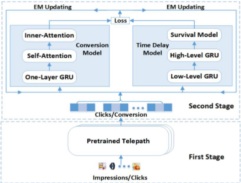
In this paper, we propose a two-stage deep neural network framework to tackle the two challenging problems in CVR prediction. To overcome the first challenge, we extract click interests from impressions by generating the dense item embedding from item images via pre-trained Telepath [Wang et al., 2017] in the first stage. Such dense item embedding is then utilized to substitute the sparse item ID features in the second stage to help alleviate the data sparsity issue. In the second stage, we propose a novel attention based conversion model to capture the fine-grained personalized product purchase interests from the sequential click data. We adopt self-attention to capture the global/high-level conversion interest patterns across all user sub-interactions. It helps to find out the hidden conversion items in click history and captures the relations among different conversion items. To tackle the time-delay challenge, we also propose a novel timedelay model. It utilizes the survival analysis to estimate the time delay and takes advantages of the post-click information to calibrate the conversion model. To train the conversion model and the time-delay model jointly on the second stage, we propose a new EM algorithm, which separates the training process of the conversion model and the delay model. We also validate the effectiveness of our two-stage deep neural network framework by conducting extensive experiments on real-world e-commerce datasets.
2 RelatedWork
Existing works mainly exploit traditional models for CVR prediction. For example, [Lee et al., 2012; Rosales et al., 2012; Chapelle, 2014] are based on logistic regression model. [Lu et al., 2017] proposed a Gradient Boosted Decision Tree (GBDT) based method. [Yang et al., 2016] and [Ji et al., 2017] tackled the problem with a graphical model. However, these traditional methods might suffer from their inherent inability in capturing the highly non-linear user behavior data, which motivates the proposal of deep learning framework. Most recently, ESMM [Xiao et al., 2018] adopted deep framework to directly extract conversion signal from impressions. However, the extremely sparse conversion can easily be overwhelmed by the click signal.
Time delay modeling is an important part of CVR prediction. There exist several works focusing on the timedelay feedback problem [Chapelle, 2014; Ji et al., 2017; Safari et al., 2017; Yoshikawa and Imai, 2018]. [Chapelle, 2014] is the first study of delayed feedback in display advertising, in which the time delay of conversion is simply assumed to be an exponential distribution. Later works either proposed other distributions such as Weibul distribution [Ji et al., 2017] or non-parametric model [Yoshikawa and Imai, 2018] to learn the delay distribution. However, all these existing methods assume a static time-delay distribution, i.e., the distribution is based on user history data before the ad click and remains unchanged regardless of post-click behaviors. In our work, we learned a dynamic time delay distribution with the abundant post-click data.
3 Model
Our proposed two-stage deep learning framework for CVR prediction is shown in Fig. 1. In the first stage, we extract click interests from impressions and utilize such impression/click information to facilitate the learning in the second stage. More specifically, we adopt the pre-trained Telepath [Wang et al., 2017] to generate the dense item embeddings from image data, which can then be utilized to substitute the sparse item ID features in the conversion model to alleviate data scarcity problem. In the second stage, we design a novel deep learning framework to extract conversion interests from clicks. Specifically, it consists of two probability models, i.e., the conversion model and the time delay model. The conversion model predicts the probability of whether a displayed ad can be finally converted after being clicked by some customer, while the time delay model captures the time delay after the click for the converted items. We jointly train the two models via our proposed EM algorithm. More details are provided in the following subsections.
3.1 ConversionModel
Conversion model is first proposed to predict the true conversion rate. Suppose that we observe a dataset D = {(Xi,Hi, yi, di, ei)}, where Xi denotes features of the candidate item, Hi represents historical clicked items of the user, yi indicates the state of candidate item, di is the time delay between the click and the conversion of the candidate, and ei is the elapsed time after the click. Specifically, Xi includes two types of features, i.e., the dense item embedding s ∈ Rn learned from item product image through Telepath [Wang et al., 2017] and the one-hot embedding o ∈ Rm to encode item category information. Then, we have Xi = (si, oi). Hi = {(sl, ol)}L1 contains L recently clicked items in chronological order. yi ∈ {0, 1} is a binary value indicating whether the candidate item has already converted. di ∈ [0,∞] is the time gap between the click and the conversion for the candidate item. If there is no conversion, then di =∞. ei ∈ [0,∞) is the elapsed time after the click, i.e., the gap of time between the click and the observation moment. Here, we use (X,H, Y,D,E) to represent the variable corresponding to each data field in D. When Y = 0 is observed, the conversion may still happen in the future due to the time delay. Thus, we use the conversion variable C ∈ {0, 1} to indicate whether the conversion of candidate item can be observed eventually.
As [Chapelle, 2014], we assume that the final conversion are only related to the characteristics of candidate item X and users behaviors H, i.e.,
It makes sense since the elapsed time E may have an influence on the observed time Y but can not affect the final conversion C. However, different from [Chapelle, 2014], we do not assume the independence between conversion time variable D and the observed time variable E.
In our conversion model, we first extract the characteristic from feature Xi of the candidate item. We align the category and dense embedding via a transformation matrix Wo ∈ Rk×m. After that, we concatenate them, followed by one fully connected layer, i.e.,
where F∗(·) is a fully connected layer with ReLU.
Another part of the conversion model is to extract the users' hidden conversion interests from the sequential user click history Hi. For each item in Hi, we adopt the similar alignment operation as candidate item, i.e., xl = concat(sl,Wool). To capture the hidden interests from the sequential history clicks, we adopt one-layer Gated Recurrent Unit (GRU) mechanism [Cho et al., 2014] to overcome the gradient vanishing problem, i.e.,
where G(·) is the GRU layer and h∗ is its hidden state.
Among the hidden information extracted by GRU from different click sub-sequences, there may exist high-level conversion interests. If there exist a conversion in a user's click history, this conversion may affect her/his click sub-sequences before next conversions. The sub-sequences before different conversions are highly correlated. To extract the global and high-level conversion interests among different hidden conversion items in history click data, we adopt the self-attention mechanism [Bahdanau et al., 2014] on top of the GRU hidden layer. Self-attention mechanism refines the representation by matching a single sequence against itself, which can capture the relationships between elements in the sequence, regardless of their distance. Before calculating the self-similarity in self-attention, we first transform the hidden state of each history item hl into query, key, and value via different fully connected layers, i.e.,
By a little abuse of notation, we denote h∗ = (h1∗ , · · · , hL∗ ). Then, we calculate the self-similarity matrix and obtain the self-attention hidden state as follows:
On the top of self-attention layer, we add the innerattention mechanism to extract the relationship between the weighted history behavior and candidate item. We calculate the similarity fraction between candidate item hidden state hc and the weighted hidden state of each history hS, i.e.,
where Wc ∈ Rs×(k+n) , WlS ∈ Rs×(k+n) , v ∈ Rs , are all the parameter matrix used in the calculation. Then, we normalize similarity scores and utilize them to align hidden state hlS , i.e.,
where α = (α1, · · · , αL), αl ∈ (0, 1), ∀l ∈ {1, · · · , L}.
In order to enhance the information fusion between the user behavior and the candidate item, we further concatenate the hidden embedding for candidate items and the hidden state vectors based on above inner/self-attention models and also their augmented matching via element-wise operations, with one fully connected layers followed, i.e.,
Finally, we can calculate the probability of item conversion based on the last hidden layer ha, i.e.,
Note that the parameters in the conversion model are cotrained with the time delay model shown in the later subsection. After training, Eq. (9) alone is used as the conversion predictor in test or online tasks.
3.2 Time DelayModel
The time delay model is then proposed to calibrate CVR prediction with additional post-click items, which refer to the clicked items of a user after the current candidate item. Denote the data set with extra post-click items as D = {(Xi,Hi, yi, di, ei, Sei )}. Here, Sei = {Sl}ei 1 is a set of post-click items during elapsed time [0, ei] with Sl as those in the l-th elapsed day. We use SE to represent the variable corresponding to feature Sei . To analyze the time delay, we first demonstrate our survival analysis framework with extra post-click items Sei , and then introduce the details of how we extract the most important information from Sei .
Survival Analysis
Survival analysis [Miller Jr, 2011] is usually conducted to analyze the survival time, especially for censored data, in which the exact survival time has not been observed, e.g., the patient may drop out of the study in the treatment. The conversions that are not observed currently can be treated as censored. Here, we leverage survival analysis to describe the time delay distribution of item conversion. We consider the survival time T as a non-negative random variable. Denote the probability density function as f(t), which indicates the probability of occurrence of events at any time t. Then, the survival time distribution function can be presented as F(t) = ∫ t 0 f(x)dx. We define the survival function as S(t) = 1 - F(t), which describes the probability Pr(T > t). We further define the hazard function h(t) as the probability of instantaneous death after the survival time t, i.e., h(t) = f(t) S(t) . Note that h(t),
f(t) and S(t) are related to each other, i.e.,
When applying survival analysis to our model, we transform it into discrete conversion delay analysis via day slots. The hazard function represents the probability that the conversion has not yet happened up to time di but happens at time di exactly. We denote the hazard function for delay time D as h(D|X, H, SE), where we ignore the hidden condition C = 1 for simplicity. Previous works usually assume that the hazard function is independent with the time E, i.e., h(D|X, H, SE) = h(D|X, H), which makes the hazard function unchanged during the period [0, ei]. Based on this assumption, the survival time distribution is simplified as,
It limits the time delay model in the scenario that the conversion rate always decreases as the time elapses. To solve this problem, we use the post-click items to infer the hazard rate h(D|Xi, Hi, Sei ) and then calculate the survival time according to Eq. 10, i.e.,
Note that when di > ei, we cannot have the post click items in period [ei, di]. Under this case, we just let h(d|Xi,Hi, Sei ) = h(ei|Xi,Hi, Sei ), ∀d ∈ {ei, · · · , di}. When di = 0, we let S(di|Xi, Hi, Sei ) = 1.
With the above survival time, we can calculate the time delay probability at time di, i.e.,
From Eq. 12 and Eq. 13, we can know that to estimate the time delay probability at time di, we need to estimate the hazard rate h(D = d|Xi, Hi, Sei ), especially for any day d ∈ {0, · · · , ei} based on the pre-click features (Xi,Hi) and the post-click data Sei . This is illustrated in next subsection.
Post-click Calibration
In our time delay model, we add the post-click information to learn the dynamic hazard function. We model the postclick information via two-level user behavior sequence between the click and the conversion and propose a two-layer GRUmodel to extract them. The first layer GRU is to extract a fixed size hidden embedding from each day slot according to the clicked items in this day slot e.g., the items Sl in day slot l ∈ {0, · · · , ei}. The second layer GRU is to extract the sequence of embedding in each day slot obtained from layer one. We consider at most N day slots, i.e., N = maxi{ei}. Compared with one-level model, which treats all clicks as one sequence, our two-level model can distinguish the conversion interests in different days and have much better ability to trace long-term interests in long click sequences. In our two-layer GRU model, we adopt the same GRU structure as in Eq. 3. Furthermore, we denote the feature of click item j in Sl during day slot l as (slj , olj ). Similar to previous operation, we combine the item embedding and category index one-hot embedding via xlj = concat(slj ,Woolj ). Then, we have the first layer feature extraction as:
We use the last hidden embedding state as the representation of day slot l, denoted as hl1 . With the first layer embedding, we can further extract the post-click information via the second layer GRU, i.e.,
Note that there may exist some day slot with empty click item. Here, we just assign them the zero embedding. For the second layer of GRU, we denote hp(e) = h2(e) to represent the hidden embedding from post-click data before day slot e ∈ {0, · · · , ei}. Combined with the embedding of candidate item hc and the hidden state embedding extracted from click history, denoted as he, we can obtain the final embedding via one fully connected layer, i.e.,
Finally, we can obtain the hazard rate as follows,
3.3 Learning Algorithm
In this subsection, we introduce the learning algorithm. Note that, the variable Y cannot be applied as labels directly due to the time delay problem. Here, we propose a novel Expectation-Maximization (EM) algorithm, which is widely used to find the maximum likelihood estimation of parameters in probabilistic models that depend on unobservable hidden variables. The intuition behind the EM algorithm in this paper is that we treat variable C as the hidden variable. More specifically, we use current probability model to calculate the expectation of C in E-step, treat the expectation of C as a new label for training in M-step.
E-step calculation: In E-step, we calculate the expectation of C by considering the estimation in two different data sets. Define the unobserved conversion data set as I0 = {i|yi = 0, ∀yi ∈ D} and the observed conversion data set as I1 = {i|yi = 1, ∀yi ∈ D}. Denote the expectation for sample i as wi. For any sample i ∈ I1, we can infer C = 1 directly, i.e.,
For any sample i ∈ I0, we cannot observe the conversion currently, but may still observe it in the future. Given the feature information (Xi, Hi, Sei ), we can estimate the expectation of C given Y = 0, i.e.,
M-step optimization: In M-step, we analyze the loglikelihood loss of data set I1 and I0 separately. We first analyze the probability of a conversion event. Given the sample i ∈ I1 with feature set (Xi, Hi, Sei ), we have:
Note that the third equality is based on the hypothesis proposed in Eq. 1. The last equality is based on the conversion probability in Eq. 9 and the time delay probability in Eq. 13.
For any i ∈ I1, we can obtain the log-likelihood easily as wi = 1 according to the conversion probability above. Then, the log-likelihood loss for I1 can be expressed as:
For the sample i ∈ I0, we can not assert whether the click will be converted eventually. We separate the case of conversion C = 1 and non-conversion C = 0. Similar to Eq. 20, we can calculate the probability of Pr{Y = 0,C = 1|Xi,Hi, Sei } and Pr{Y = 0,C = 0|Xi,Hi, Sei }. Based on the expectation value wi in E-step, we can obtain the log-likelihood function for samples in I0 as:
where we denote ˜ wi = 1 - wi.
At last, we simplify the summation of the log-likelihood loss L0 and L1, and obtain the total loss as follows:
where ti = ei if yi = 0 and ti = di otherwise. Note that we can separate the loss in Eq. 23 into two parts, one only including the parameters Θc from conversion model and the other only including the parameters Θt from time delay model. We can optimize the parameters Θc and Θt separately via updating their gradients separately.
Complexity analysis: The GRU layer takes O((n + k)2L). The Self-attention takes O((n + k)sL2 ). The inner-attention takes O((n + k)sL). Two-layer GRU takes O((n + k)2LN). When simplifying the calculation, the total complexity of our model is O((n+k)L(sL+(n+k)N 2 )(‖I0‖+‖I1‖)), where n, k, L and s are constants shown in Eq. 6 and N is the largest post-click day slot.
| Dataset | Training | Testing | ||
|---|---|---|---|---|
| # Items | # Classes | # Samples | # Samples | |
| WP1 | 69000 | 3894 | 247627 | 33703 |
| WP2 | 26467 | 3691 | 73952 | 11202 |
| JD-MP | 110445 | 3999 | 415270 | 68415 |
4 Experiments
4.1 Experimental Settings
Datasets: We evaluate our models in three data sets from JingDong ad platform 1 , summaried in Table 1. Specifically, the first two sets are users' behaviors collected from two different ad positions in Wechat (abbreviated as WP1, WP2). The last one is from JingDong middle page (short for JDMP). All training sets consist of one week data from 201809-04 to 2018-09-10, while the testing sets consist of one day data on 2018-09-12. In addition, we use the post-clicks from 2018-09-04 to 2018-09-10 in JingDong App.
Baselines: To verify the effectiveness of our two-stage deep learning framework (short for TS-DL), we choose the following baselines for comparison. To assure fairness, all baselines utilize the item embeddings from the first-stage of TS-DL.
- DFM [Chapelle, 2014]: This is the classic study of delayed feedback in display advertising, in which the time delay is assumed to be an exponential distribution.
- DIN [Zhou et al., 2018]: This baseline applies the attention mechanism to capture users' long-term interests, originally designed for CTR prediction.
- Wide&Deep [Karatzoglou et al., 2016]: This baseline is the classical work of applying deep learning models to YouTube recommendations.
- GRU+Att: This baseline utilizes GRU to model users' sequential behaviors and an attention module for capturing user interests from historical behaviors.
- TS-DL/X: This refers a series of baselines extracted from our TS-DL. The notation "/" means removing some component from our model. X refers such component, which includes {I, S, D} indicating first-stage image embedding, self-attention, and delay model accordingly.
Parameter Settings: The dimension of the dense item embedding from Telepath [Wang et al., 2017] is set as n = 50. The sparse one-hot category embedding is compressed into a dense k = 8 dimension vector. Note that candidate items, historical clicked items and post-clicked items have their own transformation matrix respectively, but with the same dimension setting. When exploiting the users click history, we only consider their L = 10 latest clicked items. We train each model up to 30 epochs, and select the results from the epoch with the highest AUC score. The batch size is set as 1024 during the training. We choose the learning rate as 0.0001 unless otherwise specified. We implement our TS-DL model and all baselines with TensorFlow [Abadi et al., 2016], and use Adam Optimizer to optimize the loss function.
1 https://jzt.jd.com/gw/adsource.htm
| Models | WP1 | WP2 | JD-MP | |||
|---|---|---|---|---|---|---|
| AUC | RelaImpr | AUC | RelaImpr | AUC | RelaImpr | |
| DFM | 0.6560 | -21.45% | 0.5795 | -22.14% | 0.6181 | -19.71% |
| DIN∗ | 0.6986 | 0.00% | 0.6021 | 0.00% | 0.6471 | 0.00% |
| Wide&Deep | 0.6573 | -20.80% | 0.6020 | -0.10% | 0.5621 | -57.78% |
| GRU+Att | 0.6975 | -0.55% | 0.6205 | 18.02% | 0.6210 | -17.74% |
| TS-DL/I | 0.6618 | -18.53% | 0.5979 | -4.11% | 0.6287 | -12.51% |
| TS-DL/D | 0.7058 | 3.63% | 0.6284 | 25.76% | 0.6325 | -9.93% |
| TS-DL/S | 0.7060 | 3.73% | 0.6395 | 36.63% | 0.6567 | 6.53% |
| TS-DL | 0.7090 | 5.24% | 0.6478 | 44.76% | 0.6589 | 8.02% |
| Models | WP1 | WP2 | JD-MP | |||
|---|---|---|---|---|---|---|
| ∆rCVR | rCVR | ∆rCVR | rCVR | ∆rCVR | rCVR | |
| DFM | 0.1317 | 0.7242 | 0.1321 | 0.8420 | 0.1150 | 0.8032 |
| DIN | 0.1391 | 0.6606 | 0.1335 | 0.7883 | 0.1091 | 0.5951 |
| Wide&Deep | 0.1048 | 0.6223 | 0.0861 | 0.6890 | 0.0269 | 0.5441 |
| GRU+Att | 0.1480 | 0.6546 | 0.1408 | 0.7856 | 0.0802 | 0.6084 |
| TS-DL/I | 0.0960 | 0.7974 | 0.1483 | 1.0461 | 0.1053 | 0.8511 |
| TS-DL/D | 0.1539 | 0.6556 | 0.1591 | 0.7813 | 0.0827 | 0.6070 |
| TS-DL/S | 0.2011 | 0.7751 | 0.2516 | 1.0275 | 0.1673 | 1.0275 |
| TS-DL | 0.2303 | 0.7945 | 0.3275 | 1.0035 | 0.2526 | 0.9459 |
4.2 Overall Performance Comparisons
In this subsection, we evaluate the overall performance of our proposed TS-DL model by comparing it with various baselines comprehensively. We adopt AUC score to measures the quality of item ranking based on the predicted CVR [Fawcett, 2005]. The higher the AUC score is, the better the performance shows. Furthermore, we choose DIN as the benchmark and adopt RelaImpr [Yan et al., 2014] as the metric to measure the relative AUC improvement.
We compare various state-of-the-art baselines on three data sets in Table 2. We have the following observations. Firstly, our TS-DL model outperforms the existing state-of-the-art methods in all data sets. Particularly, TS-DL produces significant 8.02% relative AUC improvement over baseline DIN in JD-MP, and 5.24% and 44.76% in two Wechat positions accordingly. Secondly, it also illustrates the effectiveness of ablation study. For instance, some important components in our model such as time delay module are crucial for CVR prediction. More specifically, when compared with TS-DL, TS-DL/D results in impressive 1.61%, 19% and 17.95% relative AUC reductions in three ads positions accordingly.
4.3 In-depth Conversion Rate Analysis
In this subsection, we aim to answer two questions: 1) Does our model calibrate the CVR prediction accurately? 2) Can our model separate the positive and negative samples correctly? For the first one, we introduce the metric of relative CVR (rCVR), which is defined as the ratio of predicted average CVR of given data samples over the ground-truth average CVR of the testing sets. The rCVR with smaller distance to one is better. For the second one, we define the metric of positive-negative gap, i.e., the difference between the rCVR over positive samples and that over negative samples, denoted as ∆rCVR. Larger ∆rCVR means better classification ability.
Table 3 illustrates results of CVR analysis over various baselines in three data sets. We have following observations. Firstly, our TS-DL model has the best ability to separate the positive samples and the negative samples. For instance, the positive-negative gap from TS-DL is almost twice as large as that from DFM in almost all data sets. Secondly, the overall CVR prediction from all models are under-estimated since all of the relative CVR are less than one. Yet, the models with the time-delay component, e.g., DFM and our TS-DL, can indeed calibrate the relative CVR. Our TS-DL model has the most accurate average CVR prediction in all data sets.
| Dataset | DFM | TS-DL/S | TS-DL |
|---|---|---|---|
| WP1 | 0.1125/0.1071 | 0.1114/0.1033 | 0.1112/0.1028 |
| WP2 | 0.0632/0.0906 | 0.0620/0.0835 | 0.0619/0.0833 |
| JD-MP | 0.1614/0.1267 | 0.1231/0.0908 | 0.1229/0.0889 |
4.4 Time Delay Analysis
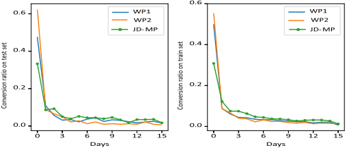
In this subsection, we compare the performance of our TS-DL model with two baselines, i.e., DFM and TS-DL/S, in predicting time delay over all three data sets, since both DFM and TS-DL/S have the time delay model. Before the detailed analysis, we first present the delay distribution on train and test data sets in Fig. 2. It shows that the number of conversions decreases with the increase of time delay. We use JensenShannon divergence [Lin and Wong, 1990] to measure the performance of the time delay prediction for different models. It is widely used to quantify the similarity of two probability distributions. The smaller the Jensen-Shannon divergence is, the more similar two distributions are. Table 4 shows the results of time delay prediction over both test and train data sets. Overall, we can observe that our TS-DL always have the smallest Jensen-Shannon divergence value over both test and train data sets. Particularly, TS-DL produces significant 23.9% and 29.8% reductions over DFM on test and train data from JD-MP accordingly.
5 Conclusions
In this paper, we proposed a novel two-stage deep learning framework to tackle the CVR prediction problem. More specifically, we extract the pre-trained embedding from impressions/clicks to assist in the conversion model. To overcome the time-delay challenge, we leverage the survival analysis to estimate the time delay via utilizing post-click information. We conduct extensive experiments with e-commerce datasets to verify the performance. The exploration of metadata such as price and brand would be in the future work.
@inproceedings{ijcai2020p487,
  title     = {An Attention-based Model for Conversion Rate Prediction with Delayed Feedback via Post-click Calibration},
  author    = {Su, Yumin and Zhang, Liang and Dai, Quanyu and Zhang, Bo and Yan, Jinyao and Wang, Dan and Bao, Yongjun and Xu, Sulong and He, Yang and Yan, Weipeng},
  booktitle = {Proceedings of the Twenty-Ninth International Joint Conference on
               Artificial Intelligence, {IJCAI-20}},
  publisher = {International Joint Conferences on Artificial Intelligence Organization},
  editor    = {Christian Bessiere},
  pages     = {3522--3528},
  year      = {2020},
  month     = {7},
  note      = {Main track},
  doi       = {10.24963/ijcai.2020/487},
  url       = {https://doi.org/10.24963/ijcai.2020/487},
}
TY - CPAPER TI - An Attention-based Model for Conversion Rate Prediction with Delayed Feedback via Post-click Calibration AU - Su, Yumin AU - Zhang, Liang AU - Dai, Quanyu AU - Zhang, Bo AU - Yan, Jinyao AU - Wang, Dan AU - Bao, Yongjun AU - Xu, Sulong AU - He, Yang AU - Yan, Weipeng T2 - Proceedings of the Twenty-Ninth International Joint Conference on Artificial Intelligence, IJCAI-20 PB - International Joint Conferences on Artificial Intelligence Organization PY - 2020 SP - 3522 EP - 3528 DO - 10.24963/ijcai.2020/487 UR - https://doi.org/10.24963/ijcai.2020/487 ER -Copied
Machine-readable versions of this paper, for tools and AI agents:





