Nearly Optimal Regret for Stochastic Linear Bandits with Heavy-Tailed Payoffs

1 Introduction

Bandit online learning is a powerful framework for modeling various important decision-making scenarios with applications ranging frommedical trials to advertisement placement to network routing [Bubeck and Cesa-Bianchi, 2012]. In the basic stochastic multi-arm bandits (MAB) [Robbins, 1952], a learner repeatedly selects one from K arms to play, and then observes a payoff drawn from a fixed but unknown distribution associated with the chosen arm. The learner's goal is to maxmize the cumulative payoffs through the trade-off between exploration and exploitation, i.e., pulling the arms that may potentially give better outcomes and playing the optimal arm in the past [Auer, 2002]. The classic upper confidence bound (UCB) algorithm achieves a regret bound of O(K log T ) over T iterations and K arms, which matches the minimax regret up to a logarithmic factor [Lai and Robbins, 1985].

One fundamental limitation of stochastic MAB is that it ignores the side information (contexts) inherent in the aforementioned real-world applications, such as the user and webpage features in advertisement placement [Abe et al., 2003], which could guide the decision-making process. To address this issue, various algorithms have been developed to exploit the contexts, based on different structures of the payoff functions such as Lipschitz [Kleinberg et al., 2008; Bubeck et al., 2011] or convex [Agarwal et al., 2013; Bubeck et al., 2015]. Among them, the stochastic linear bandits (SLB) has received significant research interests [Auer, 2002; Chu et al., 2011], in which the expected payoff at each round is assumed to be a linear combination of features in the context vector. More precisely, in each round of SLB, the learner first observes feature vector xt,a ∈ Rd for each arm a. After that, he/she selects an arm at and receives payoff rt,at , such that

∗Lijun Zhang is the corresponding author.

where θ∗ ∈ Rd is a vector of unknown parameters. The metric to measure the learner's performance is expected regret, defined as

where a∗t = argmaxa∈{1,2,...,K} x⊤t,a θ∗ and at is the action chosen by the learner at round t.

While SLB has been explored extensively [Auer, 2002; Chu et al., 2011; Abbasi-yadkori et al., 2011; Zhang et al., 2016], most of the previous work assume the payoffs are bounded or satisfy the sub-Gaussian property. However, in many real-world scenarios such as financial markets [Cont and Bouchaud, 2000] and neural oscillations [Roberts et al., 2015], the payoffs rt,a fluctuate rapidly and do not exhibit bounded or sub-Gaussian property but satisfy heavy-tailed distributions [Foss et al., 2013], i. e.,

There exists a rich body of work on learning with heavytailed distribution [Audibert and Catoni, 2011; Catoni, 2012; Brownlees et al., 2015; Hsu and Sabato, 2016; Zhang and Zhou, 2018; Lu et al., 2019], but limited work contributed to the setting of stochastic linear bandits. Medina and Yang [2016] is the first to investigate this problem, and develop two algorithms achieving ˜O(dT 2+ϵ 2(1+ϵ) ) and ˜O(√dT 1+2ϵ 1+3ϵ + dT 1+ϵ 1+3ϵ ) regret bounds respectively under the assumption that the distributions have finite moments of order 1 + ϵ for some ϵ ∈ (0, 1]. Later, Shao et al. [2018] improve these bounds to ˜O(dT 1 1+ϵ ) by developing two more delicate algorithms. When the variance of payoff is finite (i. e., ϵ = 1), this bound becomes ˜O(d√T), which is nearly optimal in terms of T. However, when the number of arms is finite, this upper bound is sub-optimal as there exists an O(√d) gap from the lower bound Ω(√dT) [Chu et al., 2011]. Thus, an interesting challenge is to recover the regret of O(√dT) under the heavytailed setting for linear bandits with finite arms.

To the best of our knowledge, this is the first work which investigates heavy-tailed SLB with finite arms and our contributions are highlighted as follows:

• We propose two novel algorithms to address the heavytailed issue in stochastic linear bandits with finite arms. One is developed based on median of means, and the other adopts the truncation technique. Furthermore, we establish an ˜O(d 12 T 1 1+ϵ ) regret bound for both algorithms.
• We provide an Ω(d ϵ 1+ϵ T 1 1+ϵ ) lower bound for heavytailed SLB problem, which matches our upper bound in terms of the dependence on T. It also implies the dependence on d in our upper bound is optimal up to a logarithmic term when ϵ = 1.
• We conduct numerical experiments to demonstrate the performance of our algorithms. Through comparisons with existing work, our proposed algorithms exhibit improvements on heavy-tailed bandit problem.

2 RelatedWork

In this section, we briefly review the related work on bandit learning. The p-norm of vector x ∈ Rd is ‖x‖p = (|x1|p + . . . + |xd|p )1/p and the ℓ2-norm is denoted as ‖·‖.

2.1 Bandit Learning with Bounded/Sub-Gaussian Payoffs

The celebrated work of Lai and Robbins [1985] derived a lower bound of Ω(K logT) for stochastic MAB, and proposed an algorithm which achieves the lower bound asymptotically by making use of the upper confidence bound (UCB) policies. Auer [2002] studied the problem of stochastic linear bandits, and developed a basic algorithm named LinRel to solve this problem. However, he failed to provide a sublinear regret for LinRel since the analysis of the algorithm requires all observed payoffs so far to be independent random variables, which may be violated. To resolve this problem, he turned LinRel to be a subroutine which assumes independence among the payoffs, and then constructed a master algorithm named SupLinRel to ensure the independence. Theoretical analysis demonstrates that SupLinRel enjoys an ˜O(√dT ) regret bound, assuming the number of arms is finite. Chu et al. [2011] modified LinRel and SupLinRel slightly to BaseLinUCB and SupLinUCB, which enjoy similar regret bound but less computational cost and easier theoretical analysis. They also provided an Ω(√dT) lower bound for SLB. Dani et al. [2008] considered the setting where the arm set is infinite, and proposed an algorithm named ConfidenceBall2 which enjoys a regret bound of ˜O(d√T). Later, Abbasi-yadkori et al. [2011] provided a new analysis of ConfidenceBall2, and improved the worst case bound by a logarithmic factor.

The main diffculty in bandit problem is the trade-off between exploitation and exploration. Most of the existing work take advantage of UCB to settle this issue and adopt the tool of ridge regression to estimate θ∗ [Auer, 2002; Chu et al., 2011]. The least square estimator of Chu et al. [2011] is

where Vt = [xτ,aτ ]τ∈Ψt ∈ R|Ψt|×d is a matrix of the historical contexts, Yt = [rτ,aτ ]τ∈Ψt ∈ R|Ψt|×1 is the historical payoff vector and Ψt ⊆ {1, 2, . . . , t - 1} is a filtered index set. The confidence interval for arm a at round t is

where wt,a = (αt + 1)√x⊤t,aAtxt,a,At = Id + V ⊤ t Vt and αt = O(√ln(TK)). If wt,a is small for all a ∈ {1, 2, . . . ,K}, which means the estimations for coming payoffs are accurate enough, the arm with highest upper confidence bound is played to execute exploitation. Otherwise, if there exists an arm a with wt,a large enough, arm a is played to explore more information.

2.2 Bandit Learning with Heavy-tailed Payoffs

The classic paper of Bubeck et al. [2013] studied stochastic MAB with heavy-tailed payoffs, and proposed a UCBtype algorithm which enjoys a logarithmic regret bound, under the assumption that the 1 + ϵ moment of the payoffs is bounded for some ϵ ∈ (0, 1]. They also constructed a matching lower bound. Medina and Yang [2016] extended the analysis to SLB, and developed two algorithms enjoying ˜O(dT 2+ϵ 2(1+ϵ) ) and ˜O(√dT 1+2ϵ 1+3ϵ + dT 1+ϵ 1+3ϵ ) regret bounds respectively. In a subsequent work, Shao et al. [2018] constructed anΩ(dT 1 1+ϵ ) lower bound for SLB with heavy-tailed payoffs, assuming the arm set is infinite, and developed algorithms with matching upper bounds in terms of T .

An intuitive explanation for heavy-tailed distribution is that extreme values are presented with high probability. One strategy tackling the heavy-tailed problem is median of means [Hsu and Sabato, 2016], whose basic idea is to divide all samples drawn from the distribution into several groups, calculate the mean of each group and take the median of these means. Another strategy is truncation following the line of research stemmed from Audibert and Catoni [2011], whose basic idea is to truncate the extreme values. Most of the existing work for heavy-tailed bandits develop algorithms based on median of means and truncation [Bubeck et al., 2013; Medina and Yang, 2016; Shao et al., 2018].

For heavy-tailed SLB algorithms adopting median of means, it is common to play the chosen arm multiple times and get r payoffs {rj t,at }rj=1 at each round. Different "means"

is considered in existing work [Medina and Yang, 2016; Shao et al., 2018]. The algorithm MoM [Medina and Yang, 2016] takes the median of {rj t,at }rj=1 to conduct least square estimation by one time and the subsequent algorithmMENU [Shao et al., 2018] adopts the median of means of least square estimations. More precisely, for j = 1, 2, . . . , r, the j-th estimator in MENU is

where ˜ Vt = [xτ,aτ ]t-1 τ=1 ∈ R(t-1)×d and ˜ Y j t = [rjτ ]t-1 τ=1 ∈ R(t-1)×1 . After that, the median of means of least square estimations is

where ‖x‖ ˜ At = √x⊤ ˜ Atx for x ∈ Rd and ˜ At = Id + ˜ V ⊤ t ˜ Vt . Then MENU selects the estimator

to predict the payoffs for all arms.

For heavy-tailed SLB algorithms adopting truncation, the essential difference between existing work is the term chosen to be truncated. The algorithm based on Confidence Region with Truncation (CRT) [Medina and Yang, 2016] conducts truncation on payoffs |rt,at | such that ˜ rt,at = rt,at I|rt,at |≤ηt for ηt = t 1 2(1+ϵ) and obtains the least square estimator through truncated payoffs ˜ rt,at . An improved algorithm TOFU [Shao et al., 2018] truncates the term |uiτ rτ,aτ |. More precisely, let [u1 , . . . , ud ] = ˜ A-1/2 t ˜ V ⊤ t and ui = [ui1 , ui2 , . . . , uit-1 ] for i = 1, 2, . . . , d. The truncation is oper-

ated as

where bt = O(t 1-ϵ 2(1+ϵ) ) and I{·} is the indicator function. Then the estimator of TOFU is

such that ui · ¯ Y i t = ∑t-1 τ=1 uiτ rτ,aτ I|uiτ rτ,aτ |≤bt for i = 1, 2, . . . , d.

3 Algorithms

In this section, we demonstrate two novel bandit algorithms based on median of means and truncation respectively and illustrate their theoretical guarantees. Without loss of generality, we assume feature vectors and target coefficients are contained in the unit ball, that is

Following the work of Chu et al. [2011], each of our two original algorithms is divided into basic and master algorithms. The main role of basic algorithms is providing confidence intervals via filtered historical informations, and master algorithm is responsible for ensuring the payoffs' independence.

3.1 Basic Algorithms

In the conventional setting where the stochastic payoffs are distributed in [0, 1], Chu et al. [2011] ultilized the AzumaHoeffing's inequality to get the narrow confidence interval (3). Here, we consider the heavy-tailed setting, i. e., for some ϵ ∈ (0, 1], there exists a constant v > 0, such that

Note that in this case, Azuma-Hoeffing's inequality is unapplicable as the bounded assumption is violated. The estimator (2) and confidence interval (3) are not suitable for heavytailed setting. Therefore, the challenge is how to establish a robust estimator associated with proper confidence intervals.

The existing work estimate the payoffs for all arms with a single estimator at each round [Auer, 2002; Chu et al., 2011; Medina and Yang, 2016; Shao et al., 2018], while the expeted payoff E[rt,a] depends not only on θ∗ but also on the contexts xt,a. Thus an intuitive conjecture is that it's better to take estimators adaptive to arms' contexts, and the following example confirms such conjecture.

Example 1. We assume θ∗ = [0.5, 0.5], the contextual information is xt,1 = [1, 0] for arm 1 and xt,2 = [0, 1] for arm 2. If we have two estimator ˆ θ1 t = [0.5, 0] and ˆ θ2 t = [0, 0.5], it's obvious that ˆ θ1 t is a better estimator for xt,1 as x⊤t,1 ˆ θ1 t = x⊤t,1 θ∗ and ˆ θ2 t is better for xt,2.

The above example encourages us to design estimators adaptive to contexts.

Median of Means

We first present the basic algorithm through median of means (BMM) to get confidence intervals for coming payoffs. The complete procedure is provided in Algorithm 1.

To adopt median of means in bandit learning, we play the chosen arm r times and obtain r sequences of payoffs. After that, BMM executes least square estimation for each sequence of payoffs and gets r estimators (Step 1-3). For j = 1, 2, . . . , r,

where Vt = [xτ,aτ ]τ∈Ψt ∈ R|Ψt|×d is a matrix of the historical contexts, Y j t = [rjτ,aτ ]τ∈Ψt is the historical payoff vector and Ψt ⊆ {1, 2, . . . , t-1} is an index set filtered by the master algorithm. Then, BMM selects an adaptive estimator ˆ θt,a for each arm a by taking the estimated payoffs as "means" (Step 6). More specifically, the estimator for arm a at current round is ˆ θt,a ∈ {ˆ θj t }rj=1 such that

By ulilizing median of means, BMM constructs a reliable confidence interval for the expected payoff (Step 6-7), which is

where wt,a = (αt + 1)√x⊤t,aAtxt,a, At = Id + V ⊤ t Vt and αt = O(t 1-ϵ 2(1+ϵ) ).

Algorithm 1 Basic algorithm through Median of Means (BMM)

Input: αt ∈ R+, r ∈ N, Ψt ⊆ {1, 2, . . . , t - 1}

Output: ˆ

rt,a, wt,a, a = 1, 2, . . . ,K

• 1: At ← Id + ∑τ∈Ψt xτ,aτ x⊤τ,aτ
• 2: bjt ← ∑τ∈Ψt rjτ,aτ xτ,aτ , rjτ,aτ is the j-th payoff of playing the arm aτ in round τ , j = 1, 2, . . . , r
• 3: ˆ θj t ←A-1 t bjt , j = 1, 2, . . . , r
• 4: Observe K arm features, xt,1, xt,2, . . . , xt,K ∈ Rd
• 5: for a = 1, 2, . . . ,K do
• 6: ˆ rt,a ← x⊤t,a ˆ θt,a, where x⊤t,a ˆ θt,a is the median of {x⊤t,a ˆ θj t }rj=1

• 8: end for

When compared with existing algorithms, the main difference lies in how to combine median of means with least square estimation. As we introduced in related work, MoM of Medina and Yang [2016] and MENU of Shao et al. [2018] take payoffs and the distance between different estimators as "means" respectively, while BMM takes estimated payoffs (8) as "means" and predicts coming payoffs with estimators adaptive to contexts. The theoretical guarantee for our estimators is displayed as follows. The payoffs' independence for filtered set Ψt is ensured by the master algorithm SupBMM and we will present it later.

Proposition 1. For fixed feature vectors xτ,aτ with τ ∈ Ψt in BMM, the payoffs {rjτ,aτ }τ∈Ψt , j = 1, 2, . . . , r are independent random variables which satisfy (1) and (6). Then, if αt = (12v) 1 1+ϵ t 1-ϵ 2(1+ϵ) and r = ⌈8 ln 2KT lnT δ ⌉, with probability at least 1 - δ/T , for any a ∈ {1, 2, . . . , K}, we have

Remark. The confidence interval of BMM depends on the 1+ϵ central moment of the payoff distribution, which is constructed at the cost of r times to play the chosen arm. When the payoffs admit a finite variance, i.e., ϵ = 1, our algorithm utilizes tighter confidence intervals with αt = √12v, in contrast, Chu et al. [2011] constructed confidence intervals with αt = O(√ln(TK)). The detailed proof can be found in the full paper [Xue et al., 2020].

Truncation

In this section, we develop the basic algorithm through truncation (BTC) to get confidence intervals for coming payoffs. The complete procedure is provided in Algorithm 2.

For heavy-tailed SLB algorithms adopting truncation, the key point is how to combine the least square estimation with truncation. The existing least square estimator (2) without truncation does not take use of current epoch's contexts xt,a, while Example 1 encourages us to consider adaptive estimator. The estimated payoff of Chu et al. [2011] is a linear combination of historical payoffs, i. e.,

Algorithm 2 Basic algorithm through Truncation (BTC)

where x⊤t,aA-1 t V ⊤ t = [βτ ]τ∈Ψt ∈ R1×|Ψt| depending on contexts. For the sake of designing an estimator adaptive to contexts, BTC truncates term βτrτ,aτ (Step 7) and obtains estimated payoff,

where ̂ Yt = [rτ,aτ I|βτ rτ,aτ |≤ht,a ]τ∈Ψt and ht,a is the truncation criterion. We set ht,a = ‖x⊤t,aA-1 t V ⊤ t ‖1+ϵ, and the confidence interval for the adaptive estimator ˆ θt,a = A-1 t V ⊤ t ̂ Yt is

where wt,a = (αt + 1)√x⊤t,aA-1 t xt,a and αt = O(ln(TK)t 1-ϵ 2(1+ϵ) ) (Step 9-10).

When compared with existing work, the main difference lies in the term chosen to be truncated. CRT of Medina and Yang [2016] truncates the payoff rt,at and TOFU of Shao et al. [2018] truncates the term uiτ rτ,aτ as we mentioned in related work. Since rt,at and uiτ rτ,aτ do not depend on current epoch's contexts, the estimators of CRT and TOFU are not adaptive. BTC develops an adaptive estimator ˆ θt,a by performing least square estimation with the truncated term βτrτ,aτ . Whether the confidence interval (11) is true is the main difficulty in the analysis of estimator ˆ θt,a because truncation results in a bias.

BTC requires that for some ϵ ∈ (0, 1], the 1+ϵ rawmoment of the payoffs is bounded, i. e., there is a constant v > 0, the payoffs admit

Proposition 2. For fixed feature vectors xτ,aτ with τ ∈ Ψt in BTC, the payoffs {rτ,aτ }τ∈Ψt are independent random variables which satisfy (1) and (12). If αt = ( 2 3 ln 2TK lnT δ + √2 ln 2TK lnT δ v + v) t 1-ϵ 2(1+ϵ) , then with probability at least 1 - δ/T, ∀a ∈ {1, 2, . . . ,K}, we have

Remark. The above proposition indicates that the confidence interval (11) provided by BTC is true wih high probability. BTC is less expensive when compared with TOFU of Shao et al. [2018] as A-1 t V ⊤ t can be computed online by the Sherman-Morrison formula [Golub and Van Loan, 1996] while ˜ A-1/2 t of TOFU can not. As we mentioned in related work, TOFU has to store both historical contextual matrix ˜ Vt and historical payoffs {rτ,aτ }t-1 τ=1 , while BTC only needs to store historical payoffs.

3.2 Master Algorithm

Here we display the master algorithm to settle the independence issue and establish its theoretical gurantees. The master algorithm is adapted from SupLinUCB [Chu et al., 2011] and the complete procedure is summarized in Algorithm 3.

At round t, the algorithm screens the candidate arms through S stages until an arm is chosen. The algorithm chooses an arm either when the expected payoff is close to the optimal one or when the confidence interval's width is large. More precisely, we consider three situations at each stage. If the estimation payoffs of all arms are accurate enough, which means the confidence level is up to 1/√T (Step 8), we do not need to do exploration and choose the arm maxmizing the upper confidence bound. Otherwise, we notice that the width of confidence interval at stage s is supposed to be 2-s . If ws t,at > 2-s for some at ∈ ˆ As (Step 11), we play it to take more exploration on this arm. The last situation is that we can not decide which arm to choose at current stage (Step 13), and only those arms which are sufficiently close to the optimal arm are filtered to the next stage (Step 14). The master algorithms taking BMM and BTC as subroutines are called SupBMM and SupBTC, respectively.

We notice that the updation of Ψst is associated with the historical trails in set ⋃σ<s Ψσt and ws t,a , while ws t,a only depends on contexts xt,a and xτ,aτ with τ ∈ Ψst . Thus the payoffs rτ,aτ are independent random variables for any fixed sequence of xτ,aτ with τ ∈ Ψst , which satisfies the assumptions of Propositions 1 and 2. We can deduce the following two regret bounds from Propositions 1 and 2.

Theorem 1. Assume all payoffs admit (1) and (6). Let r = ⌈8 ln 2KT lnT δ ⌉, for any δ ∈ (0, 1), with probability at least 1 - δ, the regret of SupBMM satisfies

Remark. We achieve a regret bound of order ˜O(d 12 T 1 1+ϵ ). For ϵ = 1, it reduces to an ˜O(√dT) bound, which implies that we get the same order as bounded payoffs assumption in terms of both d and T [Chu et al., 2011]. We point out that for any random variable X,

Algorithm 3 Master Algorithm (SupBMM and SupBTC)

Input: T ∈ N

• 1: S ← ⌊lnT⌋
• 2: Ψs1 ← ∅ for all s ∈ {1, 2, . . . , S}
• 3: for t = 1, 2, . . . , T do
• 4: s ← 1, ˆ A1 ← {1, 2, . . . ,K}
• 5: repeat

• 6: SupBMM: Use BMM with Ψst to calculate the width ws t,a and upper confidence bound ˆ rs t,a + ws t,a for every a ∈ ˆ As
• 7: SupBTC: Use BTC with Ψst to calculate the width ws t,a and upper confidence bound ˆ rs t,a + ws t,a for every a ∈ ˆ As
• 8: if ws t,a ≤ 1/√T ∀a ∈ ˆ As then
• 9: Choose at = argmaxa∈ ˆ As (ˆ rs t,a + ws t,a )
• 10: Keep the same index sets at all levels: Ψs′ t+1 ← Ψs′ t ∀s′ ∈ {1, 2, . . . , S}

• 12: Choose this arm at and update the index sets at all levels:

• 13: else ws t,a ≤ 2-s ∀a ∈ ˆ As

• 16: end if
• 17: until an arm at is found.
• 18: SupBMM: Play at r times and observe payoffs r1 t,at , r2 t,at , . . . , rr t,at
• 19: SupBTC: Play at and observe payoff rt,at 20: end for

where ϵ1, ϵ2 ∈ R+ and ϵ1 ≤ ϵ2. Therefore, our upper bound ˜O(√dT) also holds for the payoffs with finite higher order (ϵ > 1) central moments, and matches the lower bound of bounded payoffs up to some polylogarithmic factors.

Theorem 2. Assume all payoffs admit (1) and (12). For any δ ∈ (0, 1), with probability at least 1-δ, the regret of SupBTC satisfies

Remark. The above theorem assumes a finite 1 + ϵ raw moment of payoffs and achieves a regret bound of the same order ˜O(d 12 T 1 1+ϵ ) as Theorem 1, while Theorem 1 depends on the 1 + ϵ central moments of payoffs. Shao et al. [2018] proposed the algorithms achieving the regret bound ˜O(dT 1 1+ϵ ), so our algorithms have a better dependence on d for finitearmed SLB with heavy-tailed payoffs.

4 Lower Bound

In this section, we give the lower bound for finite-armed SLB with heavy-tailed payoffs.

Theorem 3. For any algorithm A with T ≥ K ≥ 4 and T ≥ (2d) 1+ϵ 2ϵ , let γ = (K/(T + 2K)) 1 1+ϵ , there exists a sequence of feature vectors {xt,a}Tt=1 for a = 1, 2, . . . , T and a coefficient vector θ∗ such that the payoff for each arm is in {0, 1/γ} with mean x⊤t,a θ∗. If d ≥ K, we have

Remark. The above theorem essentially establishes an Ω(d ϵ 1+ϵ T 1 1+ϵ ) lower bound associated with d and T for SLB under the heavy-tailed setting, which matches the upper bounds of Theorems 1 and 2 in the sense of the polynomial order on T. To the best of our knowledge, this is the first lower bound for finite-armed SLB with heavy-tailed payoffs. The detailed proof can be found in the full paper [Xue et al., 2020].

5 Experiments

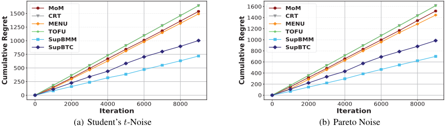
In this section, we conduct experiments to evaluate the proposed algorithms. All algorithms' parameters are set to ϵ = 1 and δ = 0.01. We adopt MoM and CRT of Medina and Yang [2016], MENU and TOFU of Shao et al. [2018] as baselines for comparison.

Let the feature dimension d = 10, the number of arms K = 20 and θ∗ = 1/√d ∈ Rd , where 1 is an all-1 vector so that ‖θ∗‖ = 1. Each element of the vector xt,a is sampled from the uniform distribution of [0, 1], and then the vector is normalized to a unit vector (‖xt,a‖ = 1). According to the linear bandit model, the observed payoff is

where ηt is generated from the following two noises.

• (i) Student's t-Noise: The probability density function of this noise is ηt ∼ Γ(2) √3πΓ(1.5) (1 + x2 3 )-2 for x ∈ R and Γ(·) is the Gamma function. Thus, the bounds of the second central moment and second raw moment of payoff are 3 and 4, respectively.
• (ii) Pareto Noise: The probability density function of this noise is ηt ∼ sxsm xs+1 Ix≥xm for x ∈ R and we set the shape s = 3 and the scale xm = 0.01. The bounds of the second central moment and second raw moment of payoff are 1 and 2.

The main difference between the above two heavy-tailed noises is that Student's t-distribution is symmetric while Pareto distribution is not.

We run 10 independent repetitions for each algorithm and display the average cumulative regret with time evolution. Fig. 1(a) compares our algorithms against algorithms of Medina and Yang [2016] and Shao et al. [2018] under Student's tnoises. Fig. 1(b) presents the cumulative regrets under Pareto noises. Our algorithms outperform MoM, CRT, MENU and TOFU with the interference of symmetric or asymmetric noises, which verifies the effectiveness of our algorithms on the heavy-tailed bandit problem. SupBMM achieves the smallest regret which is expected,since compared to SupBTC it has a more favorable logarithmic factor in regret bound.

6 Conclusion and FutureWork

In this paper, we develop two novel algorithms to settle the heavy-tailed issue in linear contextual bandit with finite arms. Our algorithms only require the existence of bounded 1 + ϵ moment of payoffs, and achieve ˜O(d 12 T 1 1+ϵ ) regret bound which is tighter than that of Shao et al. [2018] by an O(√d) factor for finite action sets. Furthermore, we provide a lower bound on the order of Ω(d ϵ 1+ϵ T 1 1+ϵ ). Finally, our proposed algorithms have been evaluated based on numerical experiments and the empirical results demonstrate the effectiveness in addressing heavy-tailed problem.

In the future, we will investigate more on closing the gap between upper bound and lower bound with respect to the dimension d.

Acknowledgments

This work was partially supported by NSFC (61976112), NSFC-NRF Joint Research Project (61861146001), and the Collaborative Innovation Center of Novel Software Technology and Industrialization.