
Learning Neural-Symbolic Descriptive Planning Models via Cube-Space Priors: The Voyage Home (to STRIPS)
Proceedings of the Twenty-Ninth International Joint Conference on Artificial Intelligence. Main track. Pages 2676-2682.
https://doi.org/10.24963/ijcai.2020/371
Keywords
- Planning and Scheduling: Planning and Scheduling
- Machine Learning: Neuro-Symbolic Methods
Abstract
We achieved a new milestone in the difficult task of enabling agents to learn about their environment autonomously. Our neuro-symbolic architecture is trained end-to-end to produce a succinct and effective discrete state transition model from images alone. Our target representation (the Planning Domain Definition Language) is already in a form that off-the-shelf solvers can consume, and opens the door to the rich array of modern heuristic search capabilities. We demonstrate how the sophisticated innate prior we place on the learning process significantly reduces the complexity of the learned representation, and reveals a connection to the graph-theoretic notion of ``cube-like graphs'', thus opening the door to a deeper understanding of the ideal properties for learned symbolic representations. We show that the powerful domain-independent heuristics allow our system to solve visual 15-Puzzle instances which are beyond the reach of blind search, without resorting to the Reinforcement Learning approach that requires a huge amount of training on the domain-dependent reward information.
- [Aineto et al., 2018] Diego Aineto, Sergio Jiménez, and Eva Onaindia. Learning STRIPS Action Models with Classical Planning. In ICAPS, 2018.
- [Amado et al., 2018] Leonardo Amado, Ramon Fraga Pereira, João Paulo Aires, Mauricio Cecilio Mag- naguagno, Roger Granada, and Felipe Meneguzzi. Goal Recognition in Latent Space. In IJCNN, 2018.
- [Asai and Fukunaga, 2018] Masataro Asai and Alex Fuku- naga. Classical Planning in Deep Latent Space: Bridging the Subsymbolic-Symbolic Boundary. In AAAI, 2018.
- [Asai and Kajino, 2019] Masataro Asai and Hiroshi Kajino. Towards Stable Symbol Grounding with Zero-Suppressed State AutoEncoder. In ICAPS, July 2019.
- [Asai, 2019] Masataro Asai. Neural-Symbolic Descriptive Action Model from Images: The Search for STRIPS. arXiv:1912.05492, 2019.
- [Bengio et al., 2013] Yoshua Bengio, Nicholas Léonard, and Aaron Courville. Estimating or Propagating Gradients through Stochastic Neurons for Conditional Computation. arXiv:1308.3432, 2013.
- [Bonet and Geffner, 2020] Blai Bonet and Hector Geffner. Learning First-Order Symbolic Representations for Plan- ning from the Structure of the State Space. In ECAI, 2020.
- [Cresswell et al., 2013] Stephen Cresswell, Thomas Leo McCluskey, and Margaret Mary West. Acquiring planning domain models using LOCM. Knowledge Engineering Re- view, 28(2), 2013.
- [Elkan and Noto, 2008] Charles Elkan and Keith Noto. Learning Classifiers from Only Positive and Unlabeled Data. In KDD. ACM, 2008.
- [Feng et al., 2018] Wenfeng Feng, Hankz Hankui Zhuo, and Subbarao Kambhampati. Extracting Action Sequences from Texts Based on Deep Reinforcement Learning. In IJCAI, 2018. IJCAI
- [Fikes and Nilsson, 1972] Richard E Fikes and Nils J. Nils- son. STRIPS: A New Approach to the Application of The- orem Proving to Problem Solving. Artificial Intelligence, 2(3), 1972. IJCAI
- [Gebser et al., 2011] Martin Gebser, Benjamin Kaufmann, Roland Kaminski, Max Ostrowski, Torsten Schaub, and Marius Schneider. Potassco: The Potsdam answer set solv- ing collection. Ai Communications, 24(2):107-124, 2011.
- [Hart et al., 1968] Peter E. Hart, Nils J. Nilsson, and Bertram Raphael. A Formal Basis for the Heuristic Determination of Minimum Cost Paths. Systems Science and Cybernetics, IEEE Transactions on, 4(2), 1968.
- [Haslum et al., 2019] Patrik Haslum, Nir Lipovetzky, Daniele Magazzeni, and Christian Muise. An Introduction to the Planning Domain Definition Language. Synthesis Lectures on Artificial Intelligence and Machine Learning, 13(2):1-187, 2019.
- [He et al., 2016] Kaiming He, Xiangyu Zhang, Shaoqing Ren, and Jian Sun. Deep Residual Learning for Image Recognition. In CVPR, 2016.
- [Helmert and Domshlak, 2009] Malte Helmert and Carmel Domshlak. Landmarks, Critical Paths and Abstractions: What's the Difference Anyway? In ICAPS, 2009. [Helmert et al., 2014] Malte Helmert, Patrik Haslum, Jörg Hoffmann, and Raz Nissim. Merge-and-Shrink Abstrac- tion: A Method for Generating Lower Bounds in Factored State Spaces. Journal of ACM, 61(3), 2014.
- [Higgins et al., 2017] Irina Higgins, Loïc Matthey, Arka Pal, et al. β-VAE: Learning Basic Visual Concepts with a Con- strained Variational Framework. In ICLR, 2017.
- [Ioffe and Szegedy, 2015] Sergey Ioffe and Christian Szegedy. Batch Normalization: Accelerating Deep Net- work Training by Reducing Internal Covariate Shift. In ICML, 2015.
- [Jang et al., 2017] Eric Jang, Shixiang Gu, and Ben Poole. Categorical Reparameterization with Gumbel-Softmax. In ICLR, 2017.
- [Koul et al., 2019] Anurag Koul, Alan Fern, and Sam Grey- danus. Learning Finite State Representations of Recurrent Policy Networks. In ICLR, 2019.
- [LeCun et al., 1998] Yann LeCun, Léon Bottou, Yoshua Bengio, and Patrick Haffner. Gradient-Based Learning Applied to Document Recognition. Proc. of the IEEE, 86(11), 1998.
- [Lindsay et al., 2017] Alan Lindsay, Jonathon Read, Joao F Ferreira, et al. Framer: Planning Models from Natural Lan- guage Action Descriptions. In ICAPS, 2017.
- [Liu et al., 2019] Liyuan Liu, Haoming Jiang, Pengcheng He, et al. On the Variance of the Adaptive Learning Rate and Beyond. arXiv:1908.03265, 2019.
- [Maddison et al., 2017] Chris J. Maddison, Andriy Mnih, and Yee Whye Teh. The Concrete Distribution: A Contin- uous Relaxation of Discrete Random Variables. In ICLR, 2017.
- [Mnih et al., 2015] Volodymyr Mnih, Koray Kavukcuoglu, David Silver, et al. Human-Level Control through Deep Reinforcement Learning. Nature, 518(7540), 2015.
- [Payan, 1992] Charles Payan. On the Chromatic Number of Cube-Like Graphs. Discrete mathematics, 103(3), 1992.
- [Richter and Westphal, 2010] Silvia Richter and Matthias Westphal. The LAMA Planner: Guiding Cost-Based Any- time Planning with Landmarks. J. Artif. Intell. Res.(JAIR), 39(1), 2010.
- [Silver et al., 2016] David Silver, Aja Huang, Chris J Mad- dison, et al. Mastering the Game of Go with Deep Neural Networks and Tree Search. nature, 529(7587):484, 2016.
- [Taddeo and Floridi, 2005] Mariarosaria Taddeo and Lu- ciano Floridi. Solving the Symbol Grounding Problem: A Critical Review of Fifteen Years of Research. Journal of Experimental & Theoretical Artificial Intelligence, 17(4), 2005.
- [Vizing, 1965] Vadim G Vizing. The Chromatic Class of a Multigraph. Cybernetics and Systems Analysis, 1(3), 1965.
- [Yang et al., 2007] Qiang Yang, Kangheng Wu, and Yunfei Jiang. Learning Action Models from Plan Examples us- ing Weighted MAX-SAT. Artificial Intelligence, 171(2-3), 2007.
References were extracted automatically from the PDF and may contain errors.
Full text extracted automatically from the PDF; figures, tables and equations may differ. The PDF is the version of record.
1 Introduction
Learning a symbolic and descriptive transition model of an environment from unstructured and noisy input (e.g. images) is a major challenge in Neural-Symbolic integration. Doing so in an unsupervised manner requires solving both the Symbol Grounding [Taddeo and Floridi, 2005] and the Action Model Learning/Acquisition problem, and is particularly difficult without reusing manually defined symbols.
Recent work that learns the discrete planning models from images has opened a direction for applying the symbolic Automated Planning systems to the raw, noisy data [Asai and Fukunaga, 2018, Latplan]. The system builds on a bidirectional mapping between the visual perceptions and the propositional states; using separate networks for modeling action applicability and effects. Latplan opened the door to applying a variety of interesting symbolic methods to real world data. E.g., its search space was shown to be compatible with symbolic Goal Recognition [Amado et al., 2018].
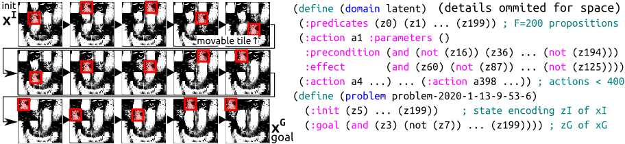
One major drawback of the previous work was that it used a non-descriptive, black-box neural model as the successor generator. Not only that such a black-box model is incompatible with the existing heuristic search techniques, but also, since a neural network is able to model a very complex function, its direct translation into a compact logical formula via a rule-based transfer learning method turned out futile [Asai, 2019]: The model complexity causes an exponentially large grounded action model that cannot be processed by the modern classical planners. Thus, obtaining the descriptive action models from the raw observations with minimal human interference is the next key milestone for expanding the scope of applying Automated Planning to the raw unstructured inputs. We propose the Cube-Space AutoEncoder (Cube-Space AE) neuro-symbolic architecture, which addresses the complexity in the action model by jointly learning a state representation and an action model of a restricted class. The purpose of the joint training is to learn an appropriate latent/state space where low-complexity action models exist, exploiting the flexibility of the end-to-end training of neural networks (NNs). The action models searched by the NN are restricted to a graph class called directed cube-like graph that corresponds precisely to the STRIPS semantics. Cube-Space AE allows us to directly extract the action effects for each action, providing a grounded PDDL [Haslum et al., 2019] that is immediately usable by off-the-shelf planners. We demonstrate its planning performance on visual puzzle domains including 15 Puzzle instances (Figure 1). Remarkably, the vast majority of states seen in the solution plans do not appear in the training data, i.e., the learned representation captures the underlying dynamics and generalizes extremely well to the individual domains studied.
2 Preliminaries
We denote a multi-dimensional array in bold and its elements with a subscript (e.g., x ∈ RN×M , x2 ∈ RM ), an integer range n < i < m by n..m, and the i-th data point of a dataset by a superscript i which we may omit for clarity. Functions (e.g. log, exp) are applied to the arrays element-wise.
Let F(V ) be a propositional formula consisting of logical operations {∧, ¬}, constants {⊤,⊥}, and a set of propositional variables V . We define a grounded (propositional) STRIPS Planning problem as a 4-tuple 〈P, A, I, G〉 where P is a set of propositions, A is a set of actions, I ⊆ P is the initial state, and G ⊆ P is a goal condition. Each action a ∈ A is a 3-tuple 〈PRE(a), ADD(a), DEL(a)〉 where PRE(a) ∈ F(P) is a precondition and ADD(a), DEL(a) are the add-effects and delete-effects, where ADD(a) ∩ DEL(a) = ∅. A state s ⊆ P is a set of true propositions, an action a is applicable when s satisfies PRE(a), and applying an action a to s yields a new successor state a(s) = (s \ DEL(a)) ∪ ADD(a).
Latplan is a framework for domain-independent imagebased classical planning [Asai and Fukunaga, 2018]. It learns the state representation and the transition rules entirely from image-based observations of the environment with deep neural networks and solves the problem using a classical planner.
Latplan is trained on a transition input X: a set of pairs of raw data randomly sampled from the environment. The ith pair in the dataset xi = (xi,0 , xi,1 ) ∈ X is a randomly sampled transition from a environment observation xi,0 to another observation xi,1 as the result of some unknown action. Once trained, Latplan can process the planning input (xI , xG), a pair of raw data images corresponding to an initial and goal state of the environment. The output of Latplan is a data sequence representing the plan execution (xI , . . . xG) that reaches xG from xI . While the original paper used an image-based implementation, conceptually any form of temporal data that can be auto-encoded to a learned representation is viable for this methodology.
Latplan works in 3 steps. In Step 1, a State AutoEncoder (SAE) (Figure 2, left) neural network learns a bidirectional mapping between raw data x (e.g., images) and propositional states z ∈ {0, 1}F , i.e., the F-dimensional bit vectors. The network consists of two functions ENC and DEC, where ENC encodes an image x to z = ENC(x), and DEC decodes z back to an image x∼ = DEC(z). The training is performed by minimizing the reconstruction loss ||x∼ -x|| under some norm (e.g., Mean Square Error for images).
In order to guarantee that z is a binary vector, the network must use a differentiable discrete activation function such as Heaviside STEP Function with straight-through estimator [Koul et al., 2019; Bengio et al., 2013] or Gumbel Softmax (GS) [Jang et al., 2017], which we use for its superior accuracy [Jang et al., 2017, Table 3]. GS is an annealing-based continuous relaxation of arg max (returns a 1-hot vector), defined as GS(x) = SOFTMAX((x-log(- log u)))/τ ), and its special case limited to 2 categories [Maddison et al., 2017] is BINCONCRETE(x) = SIGMOID((x+log u-log(1-u))/τ ), where u is a vector sampled from UNIFORM(0, 1) and τ
is an annealing parameter. As τ → 0, both functions approach to discrete functions: GS(x) → argmax(x) and BINCONCRETE(x) → STEP(x).
The mapping ENC from {. . . xi,0 , xi,1 . . .} to {. . . zi,0 , zi,1 . . .} provides the propositional transitions zi = (zi,0 , zi,1 ). In Step 2, an Action Model Acquisition (AMA) method learns an action model from zi . In Step 3, a planning problem instance (zI , zG) is generated from the planning input (xI , xG) and the classical planner finds the path connecting them. In the final step, Latplan obtains a step-by-step, human-comprehensible visualization of the plan execution by DEC'oding the intermediate states of the plan into images. For evaluation, we use domain-specific validators for the visualized results because the representation learned by unsupervised learning is not directly verifiable.
The original Latplan paper proposed two approaches for AMA. AMA1 is an oracular model that directly generates a PDDL without learning, and AMA2 is a neural model that approximates AMA1 by learning from examples, which we mainly discuss. AMA2 consists of two neural networks: Action AutoEncoder (AAE) and Action Discriminator (AD).
AAE (Figure 2, middle) is an autoencoder that learns to cluster the state transitions into a (preset) finite number of action labels. Its encoder, ACTION(zi,0 , zi,1 ), takes a propositional state pair (zi,0 , zi,1 ) as the input and returns an action. The last layer of the encoder is activated by a categorical activation function (Gumbel Softmax) to become a one-hot vector of A categories, ai ∈ {0, 1}A (∑j=A j=1 aij = 1), where A is a hyperparameter for the maximum number of action labels and ai represents an action label. For clarity, we use the one-hot vector ai and the index ai = argmaxai interchangeably. AAE's decoder takes the current state zi,0 and ai as the input and outputs z∼i,1 , acting as a progression function APPLY(ai , zi,0 ) = z∼i,1 . AAE is trained to minimize the successor reconstruction loss ||z∼i,1 - zi,1 ||.
AD is a PU-learning [Elkan and Noto, 2008] binary classifier that learns the preconditions of the actions from the observed state transitions P and the "fake" transitions U sampled by applying random actions generated by the AAE.
Combining AAE and AD yields a successor function for graph search algorithms (e.g. A∗ [Hart et al., 1968]) by enumerating the potential successor states za = APPLY(z, a) over a ∈ 1..A, then prunes the states classified as invalid by the AD. The major drawback of this approach is that both AAE and AD are black-box functions incompatible with the standard PDDL-based planners and heuristics, and thus requires custom blind search solvers.

3 Cube-Space AutoEncoder
The issue in the mathematical model of AAE is that it allows for an arbitrarily complex state transition model. The traditional STRIPS progression APPLY(s, a) = (s \ DEL(a)) ∪ ADD(a) disentangles the effects from the current state s, i.e., the effect ADD(a) and DEL(a) are defined entirely based on action a, while AAE's black-box progression APPLY(ai , zi,0 ) does not offer such a separation, allowing the model to learn arbitrarily complex conditional effects [Haslum et al., 2019]. Due to this lack of separation, the straightforward logical translation of the AAE with a rulebased learner (e.g. Random Forest) requires a conditional effect for every effect bit, resulting in a PDDL that cannot be processed by the modern classical planners due to the huge file size [Asai, 2019]. In order to make the action effect independent from the current state, we restrict the transition model learned by the network to a directed cube-like graph.
A cube-like graph G(S,D) = (V,E) [Payan, 1992] is a simple undirected graph where each node v ∈ V is a finite set v ⊂ S, D is a family of subsets of S, and for every edge e = (v,w) ∈ E, the symmetric difference d = v ⊕ w = (v \ w) ∪ (w \ v) must belong to D. For example, a unit cube is a cube-like graph because S = {x, y, z}, V = {∅, {x}, . . . {x, y, z}},E = {(∅, {x}), . . . ({y, z}, {x, y, z})},D = {{x}, {y}, {z}}. Since the set-based representation has a corresponding bitvector, e.g., V ′ = {(0, 0, 0), (0, 0, 1), . . . (1, 1, 1)}, we denote a one-to-one F-bit vector assignment as f : V → {0, 1}F . Cube-like graphs have a key difference from normal graphs.
Theorem1. (1, [Vizing, 1965]) Let the edge chromatic number c(G) of an undirected graph G be the number of colors in a minimum edge coloring. Then c(G) is either ∆ or ∆ + 1, where ∆ is the maximum degree of the nodes. (2) Mapping E → D provides an edge coloring and thus c(G) ≤ minf |D|. (3a) The minimum number of actions required to model G is c(G) with conditional effects, (3b) and minf 2|D| without.
Proof. (2) f is one-to-one: w ̸= w′ ⇔ f(w) ̸= f(w′ ). For any set X, f(w) ̸= f(w′ ) ⇔ X ⊕ f(w) ̸= X ⊕ f(w′ ). For any adjacent edges (v,w) and (v,w′ ), w ̸= w′ because G is simple (at most one edge between any nodes), thus f(v) ⊕ f(w) ̸= f(v) ⊕ f(w′ ). The remainder follows from the definition. (3a) For each edge (v, w) colored as c, we add a conditional effect to c-th action using f(v) and f(w) as the conditions and the effects (see Figure 3, left). (3b) Each d ∈ D needs 2 actions for forward/backward directions. □
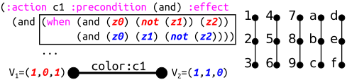
(1) and (3a,b) indicate that conditional effects can compact as many edges as possible into just A = ∆ or ∆+1 actions regardless of the nature of the transitions, while STRIPS effects cannot. In (2), equality holds for hypercubes, and there are graph instances where c(G) < minf 2|D| (Figure 3, right). We "proved" this with an Answer Set Programming solver Potassco [Gebser et al., 2011]. (Detail omitted.)
Our NN architecture is based on a directed cube-like graph, a directed extension of cube-like graph. For every edge e = (v,w) ∈ E, there is a pair of sets d = (d+, d-) = (w \ v, v \ w) ∈ D which satisfies the asymmetric difference w = (v \ d-) ∪ d+ (similar to the planning representation, we assume d+ ∩ d- = ∅). It is immediately obvious that this graph class corresponds to the STRIPS action model without preconditions. With preconditions, the state space is its subgraph. This establishes an interesting theoretical connection between our innate priors and the graph theoretic notion. We leave a formal analysis of this connection to future work.
In order to constrain the learned latent state space of the environment, we propose Cube-Space AutoEncoder. We first explain a vanilla Space AutoEncoder, an architecture that jointly learns the state and the action model by combining the SAE and the AAE into a single network. We then modify the APPLY progression to form a cube-like state space.
The vanilla Space AutoEncoder (Figure 2, right) connects the SAE and AAE subnetworks. The necessary modification, apart from connecting them, is the change in loss function. In addition to the loss for the successor prediction in the latent space, we also ensure that the predicted successor state can be decoded back to the correct image xi,1 . Thus, the total loss is a sum of: (1) the main reconstruction losses ||xi,0 - x∼i,0 ||22 and ||xi,1 -x∼i,1 ||22 , (2) the successor state reconstruction loss (direct loss) ||zi,1 - z∼i,1 ||1, (3) the successor image reconstruction loss ||xi,1 -x∼∼i,1 ||22 , and (4) the regularization loss. An important technique for successfully training the system is to employ a bootstrap phase commonly used in the literature: We delay the application of the direct loss until a certain epoch, in order to address the relatively short network distance between the two latent spaces zi,1 /z∼i,1 compared to xi,1 /x∼∼i,1 . If we enable the direct loss from the beginning, the total loss does not converge because z∼i,1 prematurely converges to zi,1 causing a mode-collapse (e.g. all 0), before the image en/decoder learns a meaningful latent representation.
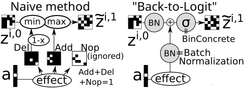
Cube-Space AE modifies the APPLY network so that it directly predicts the effects without taking the current state as the input, and logically computes the successor state based on the predicted effect and the current state. For example, a naive implementation of such a network is shown in Figure 4 (left). The EFFECT network predicts a binary tensor of F ×3, which is activated by F -way Gumbel-Softmax of 3 categories. Each Gumbel Softmax corresponds to one bit in the F-bit latent space and 3 classes correspond to the add effect, delete effect and NOP, only one of which is selected by the one-hot vector. The effects are applied to the current state either by a max/min operation or its smooth variants, smax(x, y) = log(ex + ey ) and smin(x, y) = - smax(-x, -y).
While being intuitive, we found these naive implementations extremely difficult to train. Our final contribution to the architecture is Back-to-Logit (BtL, Figure 4, right), a generic approach that computes the logical operation in the continuous logit space. We re-encode a logical, binary vector back to a continuous representation by an order-preserving, monotonic function m, so that it preserves its original meaning. We then perform the logical operation by the arithmetic addition to the continuous vector produced by the EFFECT network. Finally we re-activate the result with a discrete activation (e.g. GS/BINCONCRETE). Formally, z∼i,1 = APPLY(zi,0 , ai ) = BINCONCRETE(EFFECT(ai )+m(zi,0 )). BINCONCRETE becomes STEP after the training. Notice that it guarantees the STRIPS-style effects for the set of transitions {. . . (zi,0 , zi,1 ) . . .} generated by the same action a:
Proof. zi,1 f = STEP(m(zi,0 f ) + e) where e = EFFECT(a)f . From the assumption, 1 = STEP(m(0)+e), therefore m(0)+ e > 0. Then m(1) + e > 0 holds from monotonicity. Therefore STEP(m(zi,0 f ) + e) = 1 regardless of zi,0 f . □
This theorem allows us to extract the effects of each action a directly from the encoded states by ADD(a) = {f |∃i; zif = (0, 1)} and DEL(a) = {f |∃i; zif = (1, 0)}.
We found that an easy and successful way to implement m is Batch Normalization [Ioffe and Szegedy, 2015], a method that was originally developed for addressing the covariate shift in the deep neural networks. During the batch training of the neural network, Batch Normalization layer BN(x) takes a batched input of B vectors {xi . . . xi+B }, computes and maintains the element-wise mean and variance of the input x across the batch dimension (e.g. 1B ∑k=i+B k=i xkj for the j-th element of x), then shift and scale x element-wise so that the result has a mean of 0 and a variance of 1. We apply this to both the effect and the state vectors, i.e., APPLY(zi,0 , ai ) = BINCONCRETE(BN(EFFECT(ai )) + BN(zi,0 )).
Precondition Learning. Thanks to the strong structural prior, precondition learning with a baseline static bits extraction method turned out to be enough to plan effectively: PRE(a) = {f|∀i; zi,0 f = 1} ∪ {¬f|∀i; zi,0 f = 0} for the zi,0 satisfing ACTION(zi,0 , zi,1 ) = a. This simple procedure, which learns a single decision-rule from the dataset, achieves the sufficient success rate in the empirical evaluation. Improving the accuracy of the precondition learning is a matter of ongoing investigation.
4 Evaluation
We evaluated our approach on the dataset used by Asai and Fukunaga, which consists of 6 image-based domains. MNIST 8-Puzzle is a 42x42 pixel image-based version of the 8-Puzzle, where tiles contain hand-written digits (0-9) from the MNIST database [LeCun et al., 1998]. Valid moves in this domain swap the "0" tile with a neighboring tile, i.e., the "0" serves as the "blank" tile in the classic 8-Puzzle. The Scrambled Photograph 8-Puzzle (Mandrill, Spider) cuts and scrambles real photographs, similar to the puzzles sold in stores. LightsOut is a 36x36 pixel game where a 4x4 grid of lights is in some on/off configuration, and pressing a light toggles its state as well as the states of its neighbors. The goal is all lights Off. Twisted LightsOut distorts the original LightsOut game image by a swirl effect that increases the visual complexity. Hanoi is a visual Tower of Hanoi with 9 disks and 3 towers in 108x32 pixels. In all domains, we sampled 5000 transitions and divided them into 90%,5%,5% for the training, validation/tuning, and testing, respectively. (Code: guicho271828/latplan@Github.)
We evaluate the proposed approach via an ablation study. For each of the 6 datasets, we trained the proposed CubeSpace AE and its variants for 200 epochs, batch size 500, GS temperature τ : 5.0 → 0.7 with exponential schedule, with Rectified Adam optimizer [Liu et al., 2019]. We evaluate the network with total loss, which is the sum of the Mean Square Error (MSE) losses for the image outputs (||xi,0 - x∼i,0 ||22 + ||xi,1 - x∼i,1 ||22 + ||xi,1 - x∼∼i,1 ||22 ) and the Mean Absolute Error (MAE) direct loss for successor state prediction (||zi,1 - z∼i,1 ||1). During evaluation, Gumbel Softmax is treated as argmax without noise, following the previous work [Asai and Kajino, 2019].
| (1) BtL Cube-Space AE | (2) Total loss | (3) Ablation study | (4) Direct loss under A = 300 → 100 | ||||||||
|---|---|---|---|---|---|---|---|---|---|---|---|
| Domain | Rec. | Succ. | Direct | MinMax | Smooth | BtL | -BN | -Direct | -Succ. | Cube-Space AE | SAE+Cube-AAE |
| Hanoi | .001 | .002 | .001 | .439 | .436 | .003 | .019 | .088 | .501 | .001 → .001 | .001 → .002 |
| LOut | .000 | .000 | .000 | .506 | .506 | .000 | .002 | .239 | .412 | .001 → .008 | .010 → .040 |
| Twisted | .000 | .001 | .000 | .458 | .487 | .001 | .002 | .154 | .498 | .000 → .002 | .001 → .011 |
| Mandrill | .000 | .001 | .001 | .500 | .600 | .002 | .035 | .046 | .495 | .001 → .002 | .000 → .006 |
| Mnist | .000 | .000 | .000 | .512 | .506 | .001 | .002 | .158 | .462 | .000 → .001 | .002 → .005 |
| Spider | .001 | .001 | .001 | .607 | .563 | .003 | .026 | .073 | .376 | .003 → .002 | .001 → .003 |

We tuned the hyperparameters for the validation dataset using the sequential genetic algorithm in the public Latplan codebase (population 20, mutation rate 0.3, uniform crossover and point mutation). It selects from the learning rate r ∈ {0.1, 0.01, 0.001}, the latent space size F ∈ {100, 200, 1000}, the number of actions A ∈ {100, 200, 400, 800, 1600}, layer width W ∈ {100, 300, 600} and depth D ∈ {1, 2, 3} of ACTION/APPLY, the scaling parameter for the Zero-Suppress loss α ∈ {0.1, 0.2, 0.5} [Asai and Kajino, 2019], the variational loss β ∈ {-0.3,-0.1, 0.0, 0.1, 0.3} [Higgins et al., 2017], and the direct MAE loss γ ∈ {0.1, 1, 10}, and the bootstrap epoch for α, γ: dα, dγ ∈ {10, 20, 40, 60, 100} (scaling parameters are set to 0 before it). For each domain, we searched for 100 iterations (≈15min/iter, 24 hours total) on a Tesla K80.
We first tested several alternative architectural considerations, especially the effect of Back-to-Logit (BtL) that combines the logit-level addition and batch normalization for implementing a logical operation in the latent space. We considered 3 architectures that predict the successor state z∼i,1 . In Table 1(2), "MinMax"/"Smooth" are the variants discussed in (Figure 4, left): max(min(zi,0 , 1-DEL(a)), ADD(a)) and its smooth variants. "BtL" (Figure 4, right: proposed approach) is BINCONCRETE(BN(zi,0 ) + BN(EFFECT(a))). BtL convincingly outperformed the other options.
Next we performed an ablation study. We tested "-BN", which does not use Batch Normalization, "-direct", which relies solely on the image-based loss for predicting the successor, and "-Succ", which similarly relies solely on the statebased direct loss. Table 1(3) shows that they fail to achieve the small total loss, indicating all components are essential.
Lastly, we tested if the end-to-end training helps obtaining the compact action representation. We trained a "CubeAAE", an AAE that has the same structure as the Cube-Space AE's APPLY, but is trained on the fixed state dataset obtained by a SAE separately. Cube-AAE must learn the STRIPS effects within the fixed state representation. We tuned the hyperparameter (100 iterations) except A = 100, 300 (fixed). As A gets smaller, Cube-AAE performs significantly worse than Cube-Space AE (Table 1(4)), as expected. This is because Cube-AAE cannot model the transitions with fewer actions by reshaping the state representation to have more recurring effects, which characterize the cube-like graph.
4.1 Evaluation in the Latent Space
We ran the off-the-shelf planner Fast Downward on the PDDL files generated by our system. All domains have the fixed goal state xG. Initial states xI are sampled from the frontier of a Dijkstra search from the goal at g-value = l, the shortest path length. This makes the task harder than the l-step random walks used in previous work which allow shorter paths. In each domain, we generated 30 instances for l = 7. We tested A∗ with blind heuristics, Goal count (gc) [Fikes and Nilsson, 1972], LMcut [Helmert and Domshlak, 2009], Merge-andShrink (M&S) [Helmert et al., 2014], and the first iteration of the satisficing planner LAMA [Richter and Westphal, 2010]. In order to make sure that we have the best representation, we added 200 more genetic algorithm iterations. We compared our approach with AMA2 system (SAE+AAE+AD [Asai and Fukunaga, 2018]) with blind and gc (the only heuristics available in AMA2). Experiments are run with the 15 minutes time limit and 2GB memory limit.
| blind | gc | blind | gc | blind | gc | lama LMcut | M&S | ||||||||||||||||||
|---|---|---|---|---|---|---|---|---|---|---|---|---|---|---|---|---|---|---|---|---|---|---|---|---|---|
| f | v | o | f | v | o | f | v o | f | v | o | Domain | f | v | o | f v | o | f | v | o | f | v | o | f | v | o |
| 0 | 0 | 0 | 8 | 4 | 3 | 1 | 0 0 | 19 | 0 | 0 | LOut(30) 30 | 30 | 30 30 | 30 | 17 | 30 | 21 | 5 | 30 | 30 | 30 | 30 30 | 30 | ||
| 0 | 0 | 0 | 4 | 0 | 0 | 0 | 0 0 | 14 | 2 | 2 | Twisted(30) 30 | 25 25 | 30 | 26 | 5 | 30 | 20 | 4 | 30 | 29 | 29 | 30 | 25 | 25 | |
| 15 | 14 | 14 | 17 | 17 | 16 | 15 | 15 15 | 13 | 12 | 12 | Mandrill(30) | 30 | 29 13 | 30 | 18 | 9 | 30 | 23 | 11 | 30 | 29 13 | 30 | 30 | 13 | |
| 0 | 0 | 0 | 0 | 0 | 0 | 0 | 0 0 | 0 | 0 | 0 | Mnist(30) | 30 | 25 24 | 30 | 4 | 4 | 30 | 7 | 7 | 30 | 25 | 24 | 30 | 26 | 24 |
| 8 | 8 | 8 | 4 | 4 | 4 | 3 | 3 1 | 13 | 3 | 0 | Spider(30) | 30 | 28 | 16 30 | 27 | 12 | 28 22 | 14 | 30 28 | 16 | 30 | 28 | 16 | ||
| SAE+AAE+AD | SAE+CubeAAE+AD | 15puzzle(40) → | 32 | 32 | 29 | 28 | 9 9 | 38 | 13 | 3 38 | 38 33 | 38 | 38 | 33 | |||||||||||
Table 2 shows that our system outperforms AMA2 overall. The solutions f(ound) are v(alid) more often, and o(ptimal) with admissible heuristics. Note that, even with the admissible functions, the optimality is guaranteed only with respect to the potentially imperfect search graph generated by the Space AEs. We also observed shorter runtime / fewer expansions with the sophisticated heuristic functions like LMcut/M&S (Figure 5, column 1-2), which strongly indicates that the models we are inferring contain similar properties as the human-designed PDDL models. Also, we additionally verified the generality of the representation learned by the system. We compared the resulting plans generated by our system against the training dataset and counted how often the states/transitions could be just "memorized" from training data. Figure 5 (col. 5-6) shows that such states are rare, indicating that the planner is inducing new, unseen states/transitions. In Hanoi, the plans tend to be invalid or the goal is unreachable, even for easy instances (l = 3, v = 3, f = 32, 100 instances, blind). Hanoi requires accurate preconditions because any pair of states have only a single shortest path. Addressing its accuracy is left for future work.
Finally, we tested Mandrill 15-puzzle, a significantly more challenging 4x4 variant of the sliding tile puzzle (Figure 1). We trained the network with more hyperparameter tuning iterations (300) and a larger training set (50000). We generated l = 14, 21 instances (20 each) and ran the system (Table 2, bottom right). Blind search hits the memory limit on 6 instances which M&S, LMcut solved successfully. Figure 5 (col. 3-4) confirms the overall reduction in the node expansion and the search time. To our knowledge, this is the first demonstration of the domain-independent heuristics in an automatically learned symbolic latent space.
5 RelatedWork
Traditional action learners require the partially hand-crafted symbolic input [Yang et al., 2007; Cresswell et al., 2013; Aineto et al., 2018; Bonet and Geffner, 2020]. While some approaches extract an action model from a natural language corpus [Lindsay et al., 2017; Feng et al., 2018], they reuse the symbols in the corpus (referred to as parasitic [Taddeo and Floridi, 2005]). Our approach requires only the visual perception and can generate the propositional/action symbols completely from scratch.
While Deep Reinforcement Learning has seen recent success in settings like Atari [Mnih et al., 2015] and Go [Silver et al., 2016], it rely on the predefined action symbols in the simulator (e.g., levers, Fire button, grids). Our work compliments it by learning a simulator of the environment. While being similar to model-based RL, we generate both the transition function and the action space.
Our BtL may resemble the residual technique repopularized by Resnet [He et al., 2016], which dates back to Kalman filters st+1 = X(st) +B(ut) +w where s, u, w are the state, controller and noise, and X is sometimes an identity. The key difference is that we operate in a propositional/discrete space.
6 Discussion and Conclusion
In this work, we achieved a major milestone in propositional Symbol Grounding and Action Model Acquisition: A complete embodiment that converts the raw visual inputs into a succinct symbolic transition model in an automatic and unsupervised manner, enabling the full potential of the modern heuristic search planners. We accomplished this through the Cube-Space AutoEncoder neural architecture that jointly learns the discrete state representation and the descriptive action representation. Our main contributions are the cube-like graph prior and its Back-to-Logit implementation that shape the state space to have a compact STRIPS model.
Furthermore, we demonstrated the first evidence of the scalability boost from the state-of-the-art search heuristics applied to the automatically learned state spaces. These domainindependent functions, which have been a central focus of the planning community in the last two decades, provide admissible guidance without learning. This is in contrast to popular reinforcement learning approaches that suffer from poor sample efficiency, domain-dependence, and the complete lack of formal guarantees on admissibility.
Latplan requires uniform sampling from the environment, which is nontrivial in many scenarios. Automatic data collection via exploration is a major component of future work.
@inproceedings{ijcai2020p371,
  title     = {Learning Neural-Symbolic Descriptive Planning Models via Cube-Space Priors: The Voyage Home (to STRIPS)},
  author    = {Asai, Masataro and Muise, Christian},
  booktitle = {Proceedings of the Twenty-Ninth International Joint Conference on
               Artificial Intelligence, {IJCAI-20}},
  publisher = {International Joint Conferences on Artificial Intelligence Organization},
  editor    = {Christian Bessiere},
  pages     = {2676--2682},
  year      = {2020},
  month     = {7},
  note      = {Main track},
  doi       = {10.24963/ijcai.2020/371},
  url       = {https://doi.org/10.24963/ijcai.2020/371},
}
TY - CPAPER TI - Learning Neural-Symbolic Descriptive Planning Models via Cube-Space Priors: The Voyage Home (to STRIPS) AU - Asai, Masataro AU - Muise, Christian T2 - Proceedings of the Twenty-Ninth International Joint Conference on Artificial Intelligence, IJCAI-20 PB - International Joint Conferences on Artificial Intelligence Organization PY - 2020 SP - 2676 EP - 2682 DO - 10.24963/ijcai.2020/371 UR - https://doi.org/10.24963/ijcai.2020/371 ER -Copied
Machine-readable versions of this paper, for tools and AI agents:





