
A Bi-level Formulation for Label Noise Learning with Spectral Cluster Discovery
Proceedings of the Twenty-Ninth International Joint Conference on Artificial Intelligence. Main track. Pages 2605-2611.
https://doi.org/10.24963/ijcai.2020/361
Keywords
- Machine Learning: Clustering
- Machine Learning: Classification
Abstract
Practically, we often face the dilemma that some of the examples for training a classifier are incorrectly labeled due to various subjective and objective factors. Although intensive efforts have been put to design classifiers that are robust to label noise, most of the previous methods have not fully utilized data distribution information. To address this issue, this paper introduces a bi-level learning paradigm termed “Spectral Cluster Discovery'' (SCD) for combating with noisy labels. Namely, we simultaneously learn a robust classifier (Learning stage) by discovering the low-rank approximation to the ground-truth label matrix and learn an ideal affinity graph (Clustering stage). Specifically, we use the learned classifier to assign the examples with similar label to a mutual cluster. Based on the cluster membership, we utilize the learned affinity graph to explore the noisy examples based on the cluster membership. Both stages will reinforce each other iteratively. Experimental results on typical benchmark and real-world datasets verify the superiority of SCD to other label noise learning methods.
- [Bartels and Stewart, 1972] Richard H Bartels and George W Stew- art. Solution of the matrix equation ax+ xb= c. Communications of the ACM, 15(9):820-826, 1972.
- [Bartlett and Mendelson, 2002] Peter L Bartlett and Shahar Mendelson. Rademacher and gaussian complexities: Risk bounds and structural results. Journal of Machine Learning Research, 3(Nov):463-482, 2002.
- [Gao et al., 2016] Wei Gao, Lu Wang, Zhi-Hua Zhou, et al. Risk minimization in the presence of label noise. In Thirtieth AAAI Conference on Artificial Intelligence, 2016.
- [Gong et al., 2017] Chen Gong, Hengmin Zhang, Jian Yang, and Dacheng Tao. Learning with inadequate and incorrect supervi- sion. In 2017 IEEE International Conference on Data Mining (ICDM), pages 889-894. IEEE, 2017.
- [Gong et al., 2019] Chen Gong, Hong Shi, Tongliang Liu, Chuang Zhang, Jian Yang, and Dacheng Tao. Loss decomposition and centroid estimation for positive and unlabeled learning. IEEE Transactions on Pattern Analysis and Machine Intelligence, 2019.
- [Grubbs, 1973] Frank E Grubbs. Errors of measurement, preci- sion, accuracy and the statistical comparison of measuring in- struments. Technometrics, 15(1):53-66, 1973.
- [Han et al., 2018a] Bo Han, Jiangchao Yao, Gang Niu, Mingyuan Zhou, Ivor Tsang, Ya Zhang, and Masashi Sugiyama. Masking: A new perspective of noisy supervision. In Advances in Neural Information Processing Systems, pages 5836-5846, 2018.
- [Han et al., 2018b] Bo Han, Quanming Yao, Xingrui Yu, Gang Niu, Miao Xu, Weihua Hu, Ivor Tsang, and Masashi Sugiyama. Co- teaching: Robust training of deep neural networks with extremely noisy labels. In Advances in Neural Information Processing Systems, pages 8527-8537, 2018.
- [Huang et al., 2015] Jin Huang, Feiping Nie, and Heng Huang. A new simplex sparse learning model to measure data similarity for clustering. In Twenty-Fourth International Joint Conference on Artificial Intelligence, 2015. IJCAI
- [Jiang et al., 2017] Lu Jiang, Zhengyuan Zhou, Thomas Leung, Li- Jia Li, and Li Fei-Fei. Mentornet: Learning data-driven curricu- lum for very deep neural networks on corrupted labels. arXiv preprint arXiv:1712.05055, 2017.
- [Magoulas and Prentza, 1999] George D Magoulas and Andriana Prentza. Machine learning in medical applications. In Advanced Course on Artificial Intelligence, pages 300-307. Springer, 1999.
- [Miranda et al., 2009] André LB Miranda, Luís Paulo F Garcia, André CPLF Carvalho, and Ana C Lorena. Use of classification algorithms in noise detection and elimination. In International Conference on Hybrid Artificial Intelligence Systems, pages 417- 424. Springer, 2009.
- [Muhlenbach et al., 2004] Fabrice Muhlenbach, Stéphane Lallich, and Djamel A Zighed. Identifying and handling mislabelled instances. Journal of Intelligent Information Systems, 22(1):89- 109, 2004.
- [Natarajan et al., 2013] Nagarajan Natarajan, Inderjit S Dhillon, Pradeep K Ravikumar, and Ambuj Tewari. Learning with noisy labels. In Advances in Neural Information Processing Systems, pages 1196-1204, 2013.
- [Nie et al., 2016] Feiping Nie, Xiaoqian Wang, Michael I Jordan, and Heng Huang. The constrained laplacian rank algorithm for graph-based clustering. In Thirtieth AAAI Conference on Artificial Intelligence, 2016.
- [Northcutt et al., 2017] Curtis G Northcutt, Tailin Wu, and Isaac L Chuang. Learning with confident examples: Rank pruning for robust classification with noisy labels. arXiv preprint arXiv:1705.01936, 2017.
- [Patriksson, 2008] Michael Patriksson. On the applicability and solution of bilevel optimization models in transportation science: A study on the existence, stability and computation of optimal solutions to stochastic mathematical programs with equilibrium constraints. Transportation Research Part B: Methodological, 42(10):843-860, 2008.
- [Patrini et al., 2016] Giorgio Patrini, Frank Nielsen, Richard Nock, and Marcello Carioni. Loss factorization, weakly supervised learning and label noise robustness. In International Conference on Machine Learning, pages 708-717, 2016.
- [Patrini et al., 2017] Giorgio Patrini, Alessandro Rozza, Aditya Kr- ishna Menon, Richard Nock, and Lizhen Qu. Making deep neural networks robust to label noise: A loss correction approach. In Proceedings of the IEEE Conference on Computer Vision and Pattern Recognition, pages 1944-1952, 2017.
- [Shi et al., 2018] Hong Shi, Shaojun Pan, Jian Yang, and Chen Gong. Positive and unlabeled learning via loss decomposition and centroid estimation. In Proceedings of the 27th International Joint Conference on Artificial Intelligence, pages 2689-2695, 2018. IJCAI
- [Tanaka et al., 2018] Daiki Tanaka, Daiki Ikami, Toshihiko Ya- masaki, and Kiyoharu Aizawa. Joint optimization framework for learning with noisy labels. In Proceedings of the IEEE Conference on Computer Vision and Pattern Recognition, pages 5552-5560, 2018.
- [Wang et al., 2015] Zhangyang Wang, Yingzhen Yang, Shiyu Chang, Jinyan Li, Simon Fong, and Thomas S Huang. A joint optimization framework of sparse coding and discriminative clustering. In Twenty-Fourth International Joint Conference on Artificial Intelligence, 2015. IJCAI
- [Wei et al., 2019] Yang Wei, Chen Gong, Shuo Chen, Tongliang Liu, Jian Yang, and Dacheng Tao. Harnessing side information for classification under label noise. IEEE Transactions on Neural Networks and Learning Systems, 2019.
- [Xia et al., 2019] Xiaobo Xia, Tongliang Liu, Nannan Wang, Bo Han, Chen Gong, Gang Niu, and Masashi Sugiyama. Are anchor points really indispensable in label-noise learning? Ad- vances in Neural Information Processing Systems, pages 6835- 6846, 2019.
- [Xu et al., 2016] Chang Xu, Dacheng Tao, and Chao Xu. Robust extreme multi-label learning. In Proceedings of the 22nd ACM SIGKDD International Conference on Knowledge Discovery and Data Mining, pages 1275-1284. ACM, 2016.
References were extracted automatically from the PDF and may contain errors.
Full text extracted automatically from the PDF; figures, tables and equations may differ. The PDF is the version of record.
1 Introduction
Traditional supervised learning models such as Support Vector Machines and Deep Neural Networks usually require accurately labeled datasets for model training. However, labeling errors often occur in practice due to the human fatigue [Magoulas and Prentza, 1999], knowledge limitation [Gong et al., 2017], or measurement error of instruments [Grubbs, 1973]. Therefore, it is crucial for us to design effective training algorithms which are robust to noisy labels.
Several methods for tackling label noise have been developed so far, which can be roughly divided into two types. The methods of first type rely on data cleansing technique. The early-staged methods basically consist of two steps, namely picking up the clean data or filtering out the noisy data, and then deploying the clean data to train the classifier. For instance, neighborhood relationship [Muhlenbach et al., 2004]
was utilized to filter out the noisy examples. In [Miranda et al., 2009], different classifiers were employed to vote for the clean data. Recent data cleansing methods have focused on Deep Neural Networks. MentorNet [Jiang et al., 2017] used a self-paced curriculum to select the clean set. Coteaching [Han et al., 2018b] adopted peer networks and used the "small-loss" and disagreement behaviors of network to choose the probably reliable examples for network updating. However, all the above approaches deploy various heuristic and ad-hoc criteria to decide the clean examples with correct labels, which lack theoretical guarantees.
Therefore, the methods belonging to the second type aim to train the classifiers that are robust to label noise directly, without the need of selecting the clean examples. For example, in [Natarajan et al., 2013], an unbiased risk estimator was designed for establishing loss function, which made it possible to resist the influence of label noise and learn a robust classifier. In [Patrini et al., 2016], the loss function was factorized into two parts, in which only one part was affected by noisy labels. Consequently, they slightly modified the vanilla Stochastic Gradient Descent (SGD) during parameter optimization to reduce the impact of label noise on model training. Besides, in [Gao et al., 2016; Shi et al., 2018; Gong et al., 2019], a similar decomposition was proposed, where the label-dependent part was tackled by unbiasely estimating the labeled instance centroid. Nonetheless, these techniques can only deal with canonical binary classification problem and often require prior knowledge on noise rate or label flipping probability, which may be infeasible or inaccessible in real-world applications. In fact, several methods [Patrini et al., 2017; Northcutt et al., 2017; Han et al., 2018a] was developed for prior knowledge estimation, but their performances are often not satisfactory in the presence of high-dimensional datasets [Han et al., 2018b].
In addition, there are some other approaches for dealing with noisy labels. For instance, [Xia et al., 2019] utilized Transition-revision to designed a deep-learning-based riskconsistent estimator to accurately tune the transition matrix; [Tanaka et al., 2018] jointly trained the networks and estimated true labels, and [Wei et al., 2019] employed the row-sparse residual matrix to capture the incorrectly labeled examples. However, all the above approaches share an implicit deficiency that they have not fully utilized the data distribution information for label noise learning.
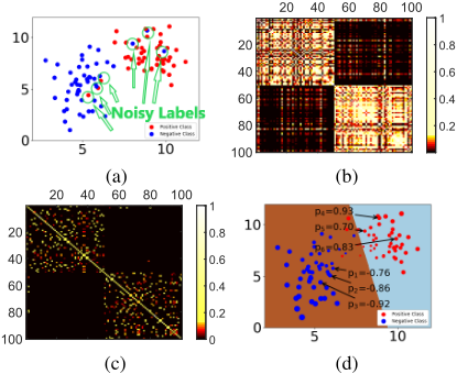
In this paper, we propose an effective learning paradigm called "Spectral Cluster Discovery" (SCD), which allows us to train a robust classifier even when the noise rate is relatively high (e.g., 60% noisy examples occur in the training set). Our idea stems from LNSI approach [Wei et al., 2019] and the observation that the examples distributed within a connected cluster are likely to have same class label. Similar to LNSI, our SCD also handle label noise in a matrix recovery fashion (Learning stage). LNSI works on a fixed pre-constructed affinity graph (Figure 1 (b)) for noise identification, which lacks adaptability during the learning process. Thus, the distribution information given by the affinity graph may be misleading. In contrast, the graph in our method will be dynamically updated (Clustering stage) according to the gradually discovered data clusters. Namely, we use the learned classifier to assign the examples with similar labels into the same connected component in the affinity graph, where each connected component represents a class of examples. Naturally, we want the number of connected component to be exactly the same as the total amount of classes. Based on the well-learned graph (Figure 1 (c)), we can then train a classifier by discovering the noisy examples whose labels are different with those in the same cluster and re-annotate them according to the cluster membership (Figures 1 (c)(d)). Moreover, we alternate between the above two stages to make sure that both the classifier and affinity graph are optimal.
Consequently, we formulate our model as a bi-level optimization problem [Wang et al., 2015], where the upper-level problem (Learning stage) is to optimize a classifier in the presence of label noise, and the lower-level problem (Clustering stage) is to exploit the spectral clusters for graph updating. The two problems are iteratively solved and are also benefited from each other, so that a robust classifier can be finally established. Theoretically, we prove that the generalization error of the induced classifier is upper bounded. Experimentally, we compare our proposed SCD with other state-of-the-art label noise learning algorithms on several popular datasets, and the results verify the superiority of SCD to other typical methods.
2 Problem Setup
Let (x1, y1), (x2, y2), · · ·, (xn, yn) be n training examples identically and independently (i.i.d) drawn from an underlying (noise-free) distribution D over X × Y, where X ⊆ Rd denotes the feature space of dimension d, and Y ⊆ {0, 1}c denotes the c-dimensional label space with c being the number of classes. Conventionally, we represent the class label of each data as a "1-of-c" indicator vector y = (y1 , y2 , ···, yc )⊤, where yk = 1 if the corresponding example x belongs to the k-th class and yk = 0 otherwise. Therefore, traditional supervised learning algorithm aims to design a classifier f ′ : X → Y which is able to classify any unseen test example x ∈ Rd to one of the c classes.
However, in label noise learning, the examples from clean distribution D are unavailable. Before being observed, random classification noise are injected into training examples and what we can obtain are the corrupted examples (x1, ˜y1), (x2, ˜y2), · · ·, (xn, ˜yn) drawn from the noisy distribution ˜D over X × ˜ Y, where ˜ Y ⊆ {0,1}c denotes the noisy label space while X ⊆ Rd remains the same, then our goal is to train a robust classifier f that can achieve accurate classification in the presence of noisily labeled training examples. In the rest of the paper, we denote a matrix M with bold capital letter and denote Mi as the i-th column of matrix M.
3 Model Establishment
As is mentioned in the introduction, SCD alternates between learning a robust classifier in the presence of label noise (i.e. Learning stage) and discovering data clusters in the training set (i.e. Clustering stage) to aid noise correction, in which the latter is the core of SCD to boost the learning performance. Next we will detail our SCD algorithm.
Learning Stage. The function of Learning stage is to learn a classifier in the presence of label noise (Figures 1 (a)(d)), by optimizing the low-rank approximation of the groundtruth label martrix. Let X = (x1, x2, · · ·, xn) ∈ Rd×n and ˜Y = (˜y1, ˜y2, · · ·, ˜yn) ∈ Rc×n denote the feature matrix and the noisy label matrix, respectively, and we decompose ˜Y as ˜Y = Y + E = W⊤X + E, in which the ground-truth label matrix Y ∈ Rc×n can be recovered by the projection matrix W ∈ Rd×c of the classifier f, and the error matrix E ∈ Rc×n measures the difference between the observed label matrix and the ground-truth label matrix. Moreover, it is reasonable to assume that the ground-truth label matrix can be well approximated by a low-dimensional subspace [Xu et al., 2016], so we encourage the ground-truth label matrix W⊤X to be low-rank by employing matrix factorization, i.e. W = UV [Xu et al., 2016], where U ∈ Rd×r and V ∈ Rr×c (r controls the maximal rank of W⊤X). Besides, we hope that the number of non-zero columns of error matrix E is small since the label noise in training examples is usually sparse [Wei et al., 2019], so we minimize the ℓ2,1 norm ‖E‖2,1 = ∑ni=1 ‖Ei‖2. Moreover, to fulfill the assumption that similar examples should have similar labels, we further introduce the graph Laplacian regularizer. Define an affinity matrix S ∈ Rn×n , with the (i, j)-th entry (i.e. sij) computed by sij = exp(-‖xi - xj‖2 /(2σ2 )) ( σ is Gaussian kernel width), and sij measures the similarity between xi and xj. The graph Laplacian matrix L ∈ Rn×n can then be computed based upon S as L = D- (S⊤ +S)/2 where D ∈ Rn×n is a diagonal degree matrix with the i-th diagonal element defined by dii = ∑j sij . Therefore, the Learning stage is formulated
where "Tr(·)" computes the trace of the corresponding matrix, λ1, λ2 and λ3 are nonnegative trade-off parameters. However, this formulation depends on a fixed pre-constructed affinity matrix S for noise identification, which can be inaccurate and also lacks adaptability during the learning process.
Clustering Stage. The function of Clustering stage is to aid the Learning stage. To this end, this stage builds an ideal block diagonal affinity graph which is able to help the Learning stage to discover and correct noisy examples. Specifically, if the label of an example is different from its companion in the same connected component, then its label are probably wrong. Thus, we re-annotate this examples based on its cluster membership, so that the robust classifier can be trained (Figures 1 (c)(d)).
In order to learn such an affinity matrix, we strictly constrain the rank of the graph Laplacian matrix to be n - c to make sure that the affinity graph will contain exactly c connected components [Nie et al., 2016]. Meanwhile, we assume that the examples with similar labels should have larger sij than those with dissimilar ones. To avoid trivial solution, the sum of each column of S is constrained to be 1 (i.e. S⊤i 1 = 1, where 1 denotes the all-one column vector). Further, the affinity matrix should be nonnegative, so the Clustering stage is formulated as
where Ls denotes the graph Laplacian matrix computed by a learned affinity matrix S instead of a pre-constructed one, µ is a nonnegative trade-off parameter, and ‖S‖2F is minimized to avoid over-fitting. By solving problem (2), we will establish an ideal affinity graph that can benefit the Learning stage, so we apply the learned affinity matrix S to problem (1), by substituting L by Ls. After that, we can obtain the cluster membership for each example according to the ground-truth label matrix.
However, if we do not have access to the true labels of all training examples before we build such an affinity graph, the result may not be satisfactory. That being said, we may assign the examples with noisy label to the wrong connected component because we are misguided by that inaccurate information. To address this issue, we utilize the Learning stage to help the Clustering stage. Namely, we integrate the Clustering stage (i.e. problem (2)) to the Learning stage (i.e. problem (1) by which we can dynamically build an adaptive affinity matrix and learn a robust classifier according to the gradually explored data clusters (Figures 1 (b)(c)).
To achieve this effect, our SCD paradigm is finally formulated as a bi-level optimization problem as
︷︷ Lower-level poblem: Clustering stage
The upper-level problem (which is directly related to label noise learning) can guide the lower-level problem (which boosts label noise learning) to gradually explore the true data clusters, meanwhile the lower-level problem is helpful for the upper-level problem to progressively discover the noisy examples whose labels are different from those in the same connected component, and train the robust classifier. Consequently, these two procedures can be benefited from each other and dynamically work together to acquire good learning result. Besides, according to the Weierstrass Theorem in [Patriksson, 2008], it can be easily verified that our bi-level model (3) satisfies the conditions which are sufficient for a bi-level problem to have an optimal solution.
4 Optimization
In this section, we present the detailed solution for optimizing the SCD parameters in the bi-level formulation (3), which alternatively optimizes between the upper-level problem and the lower-level problem mentioned above.
4.1 Upper-level ProblemOptimization
The upper-level problem (i.e. Learning stage) can be iteratively solved by sequentially updating U, V and E by solving their respect subproblem. After taking the derivative of subproblem regarding U w.r.t. U, and denoting (·)† as the pseudo-inverse of the corresponding matrix, we can update U by solving the following Sylvestor equation [Bartels and Stewart, 1972]
By denoting I as the identity matrix with proper size throughout this paper, then we have
4.2 Lower-level ProblemOptimization
The lower-level problem (i.e. Clustering stage) defined in Eq. (2) is difficult to solve due to the rank constraint, so necessary ways should be found to relax it. According to [Nie et al., 2016], given a large enough ρ, the lower-level problem is equivalent to the following problem:
When S is fixed, the problem (7) becomes:
The solution of the above optimization problem can be easily obtained by setting the columns of F equal to the c smallest eigenvectors of Ls [Nie et al., 2016]. When F is fixed, with Fk being the k-th column of F, the columns of S can be separately updated in parallel by solving
By denoting wij = ‖(UV)⊤xi - (UV)xj‖22 and bij = ‖Fi - Fj‖22 as the j-th element of Wi and Bi, and also denoting Vi = - µ2 Wi - ρ2 Bi, then based on [Huang et al., 2015], sij has a closed-form solution as
where Zi = Vi - 11⊤ n Vi + 1n 1 and q∗ i can be obtained by solving f(qi) = 1n ∑nj=1 (q∗ i - uij)+ - qi = 0 with Newton method.
After that, we update the graph Laplacian matrix via Ls = D- (S⊤ +S)/2, for the next iteration. After the algorithm converges, we can obtain the parameter of robust classifier by W∗ = U∗V∗ and label y of any given example x can be computed by y = argmaxi(W∗⊤x)i. The complete algorithm is summarized in Algorithm 1, from which we see that our SCDmodel (Eq. (3)) can be easily trained.
For time complexity, in line 8 of Algorithm 1, the Sylvester equation for optimizing U is solved by Bartels-Stewart algorithm that takes O((max{d, c})3 ) complexity. Next, we update V by computing the inverse of a c × c matrix in line 9, and the time complexity is O(c3 ). The computation of the ℓ2 norm of every column of E in line 10 requires O(nc) complexity. Moreover, in line 14, we search for q∗ i for every column Si of S by Newton method, of which the time complexity is O(nlogn). Finally, computing the eigenvectors of F takes O(n3 ) complexity. Therefore, the total complexity of the proposed model is O (T1([max{d, c}]3 + c3 +nc) +T2(nlogn+n3 )), by assuming that the upper-level and lower-level optimizations are iterated for T1 and T2 times, respectively. Since SCD often converges in a few iterations, the time complexity is acceptable.
5 Theoretical Analysis
This section analyzes the generalizability of our proposed SCD. SCD aims to learn an decision function fθ : X → ˜ Y
Algorithm 1 The algorithm for solving SCD
- 1: Input: Feature matrix X, corrupted label matrix ˜Y, trade-off parameters λ1, λ2, λ3, µ;
- 2: Randomly generate an affinity matrix S.
- 3: Initialize U=O, V =O, E =O; Set ρ = 1000;
- 4: Set iter = 0
- 5: repeat
- 6: // Learning stage
7:
repeat
8:
Update U via Eq. (4);
9:
Update V via Eq. (5);
- 10: Update E via Eq. (6);
- 11: until Learning stage has converged;
- 12: // Clustering stage
- 13: repeat
- 14: Update S via Eq. (10);
15:
Update F via solving Eq. (8);
- 16: until Clustering stage has converged;
- 17: // Update graph Laplacian matrix
- 18: Ls =D- (S⊤ +S)/2;
- 19: iter := iter + 1;
- 20: until SCD has converged.
- 21: Output: Optimal parameter of robust classifier W∗ = U∗V∗ .
which is controlled by θ = (W,E). Let Θ = {(W,E) : rank(W) ≤ k, ‖W‖F ≤ A, ‖E‖2,1 ≤ E2,1} and FΘ be the feasible solution set of θ and the feasible solution set of fθ, respectively. In order to find the optimal f ∗ θ , SCD minimizes the empirical ℓ-risk as
Let Rℓ(f) = E(x,y)[ ˜Rℓ(f)] be the expected ℓ-risk, then our goal is to show that the empirical ℓ-risk will converge to the expected ℓ-risk when n is sufficiently large. As is shown in [Bartlett and Mendelson, 2002], the Rademacher complexity is an useful tool for analyzing the bound of the generalization error of SCD, therefore we present the definition of Rademacher complexity as follows. Denote
as the Rademacher complexity of the function class F on X and
as the empirical Rademacher complexity on the training set, where σi ∈ {-1, 1}(i = 1, 2, · · · , n) are independent uniform Rademacher random variables, then the Rademacher complexity of our model can be written as [Xu et al., 2016]
By defining
and
we have
so we should analyze R(1) n (FΘ) and R(2) n (FΘ), respectively. Given the optimal S∗ , and for any S which is not optimal but meets the constraints in the lower-level problem, we can prove that
which leads to
According to [Wei et al., 2019], we know that
where λmin(·) denotes the minimal eigenvalue of the corresponding matrix. Combining Eq. (19) and Eq. (20), and denoting WF = √ 1µ (n+2µ(n- c))/λmin(XL∗sX)⊤, we
By defining ¯x = ∑ni=1 σixi, and arranging c copies of ¯x as a d × c matrix ¯X = (¯x, ¯x, · · ·, ¯x), we have
Then we have the following lemma:
Lemma 1. ([Xu et al., 2016]) Let ΘW = {W : rank(W) ≤ k, ‖W‖F ≤ WF}, ‖¯X‖F ≤ XF and ‖xi‖2 ≤ X2, then the Rademacher complexity R(1) n (FΘ) is upper bounded by:
Nowwe introduce another useful lemma.
Lemma 2. ([Wei et al., 2019]) Let ΘE = {E : ‖E‖2,1 ≤ E2,1}, R(2) n (FΘ) is upper bounded by
Based on Lemma 1 and Lemma 2, we can easily derive the bound of the expected ℓ-risk, namely
Theorem 1. Let ℓ be the loss function bounded by B with Lipschitz constant Lℓ, and δ be a constant where 0 < δ < 1. Then with probability at least 1-δ, we have
This inequality can be easily derived based on Lemma 1 and Lemma 2. Theorem 1 indicates that the expected loss is upper bounded. Specifically, WF and E2,1 are related to the learned affinity matrix and the error matrix, respectively. If the minimal eigenvalue of XL∗sX⊤ is large or the noise rate is small (i.e. E2,1 is small), the upper bound of the expected ℓ-risk in the righthand side of Eq. (26) will be reduced.
| Dataset | #exapmles | #classes | #features |
|---|---|---|---|
| Zoo | 101 | 7 | 16 |
| Seed | 210 | 3 | 7 |
| Haberman | 306 | 2 | 3 |
| Ionosphere | 351 | 2 | 34 |
| German | 1000 | 2 | 24 |
6 Experiment
In this section, we compare SCD with several representative methods on a number of real-world collections, and also study the parametric sensitivity of SCD.
6.1 Experiments on UCI Benchmark Dataset
We compare SCD with four baseline algorithms on six UCI benchmark datasets including Zoo, Seed, Haberman, Ionosphere, and German, whose attributes are summarized in Table 1. Note that 80% of the examples in each dataset are randomly chosen to establish the training set, and the remaining 20% examples in each dataset are served as test set. To incorporate different noise rate to the training sets, we randomly pick up 0%, 20%, 40%, and 60% examples from the training sets and inject symmetric noise [Patrini et al., 2016] to these selected examples. Such contamination and partition are conducted five times, so the accuracies are the mean values of the outputs of five independent trials.
The baselines include: 1) Unbiased Logistic Estimator (ULE) [Natarajan et al., 2013], 2) µ Stochastic Gradient Descent (µSGD) [Patrini et al., 2016], 3) Labeled Instance Centroid Smoothing (LICS) [Gao et al., 2016], 4) Rank Pruning (RP) [Northcutt et al., 2017], and 5) Label Noise handling via Side Information (LNSI) [Wei et al., 2019]. Note that the first three approaches are designed for binary classification tasks, so we use the one-vs-rest strategy to apply them to multi-class cases. For fair comparison, the prior knowledge such as noise rate is provided for all methods, and LNSI is implemented on a 10-NN graph with Gaussian kernel width σk = 0.5.
The classification accuracies of all compared methods on the test set are presented in Figure 2. We observe that SCD yields better performance than other baselines in most cases. Especially, when the noise rate increases, the accuracies of most baselines decrease, but SCD still performs robustly.
6.2 Experiment on Real-world Datasets
We use ISOLET dataset and CIFAR-10 dataset to demonstrate the superiority of SCD in dealing with different kinds of practical problems. First, we address a speech recognition task based on the ISOLET dataset which contains 150 subjects that are required to pronounce each letter in the alphabet (i.e. from"A" to "Z") twice. The dataset consists of 7797 examples with 617 dimensions. The way for partitioning the training set and test set is the same as previous experiments, and we also vary the noise rate from 0% to 60%. From Table 2, it can be observed that SCD achieves better classification result than other baselines, and is more robust than other methods when the noise rate increases.
Second, we use CIFAR-10 to validate the ability of SCD on processing image data, which contains 60000 natural images across 10 classes. In our experiment, we randomly pick up 30000 image examples form CIFAR-10 across different classes. The resolution of each image is 32×32×3. Other experimental settings are the same as before. The classification accuracies of all the compared approaches under different noise rates are shown in Table 3. It can be observed that SCD outperforms other methods and is robust with the increase of the noise rate. Note that LICS is not involved as it is not scalable to CIFAR-10 dataset.

| Method | 0% | 20% | 40% | 60% |
|---|---|---|---|---|
| ULE µSGD LICS RP LNSI SCD | 0.823±0.104✓ 0.796±0.020✓ 0.883±0.022✓ 0.965±0.005 0.891±0.006 0.914±0.003 | 0.747±0.060✓ 0.744±0.021✓ 0.758±0.048✓ 0.838±0.007✓ 0.823±0.006✓ 0.917±0.006 | 0.618±0.079✓ 0.470±0.047✓ 0.615±0.060✓ 0.716±0.011✓ 0.821±0.012✓ 0.911±0.016 | 0.417±0.078✓ 0.475±0.037✓ 0.442±0.052✓ 0.557±0.001✓ 0.805±0.019✓ 0.884±0.015 |
6.3 Parametric Sensitivity
Note that the objective function Eq. (3) in our method contains four trade-off parameters λ1, λ2, λ3 and µ that should be manually tuned. Therefore, it is necessary to discuss whether the choices of them will significantly influence the performance of SCD. To this end, we examine the classification accuracy of SCD on test set at two different noise rates (20% and 60%) via changing one of λ1, λ2, λ3 and µ, and meanwhile fixing the others to the optimal constant values under different datasets and different noise rates (i.e. λ∗1 = 10-3 , λ∗2 = 101 , λ∗3 = 101 and µ∗ = 10-3 for both noise rate 20% and 60%).
The ISOLET dataset is used for the parametric sensitivity analysis. Table 4 shows the variation of accuracies w.r.t. the four trade-off parameters on ISOLET dataset.
As is shown in Table 4, SCD is robust to the variations of all the trade-off parameters in a wide range, so they can be easily tuned for practical use. Besides, we learn that λ1 and µ are preferred to be small; while λ2 and λ3 are suggested to choose a relatively large number.
7 Conclusion
In this paper, we propose a novel bi-level paradigm to solve the label inaccuracy problem. Specifically, we utilize the distribution information of the dataset by learning an adaptive affinity graph which is ideally block diagonal, and integrate it to the learning of the robust classifier. Moreover, the learned classifier can help the learning of the affinity graph, in which way this two stages mutually complement to each other. We devise the optimization algorithm for the proposed SCD. Experimental results on several typical datasets reveal that SCD generally obtains higher classification accuracies than existing state-of-the-art label noise learning methods.
| Method | 0% | 20% | 40% | 60% |
|---|---|---|---|---|
| ULE µSGD RP LNSI SCD | 0.823±0.104✓ 0.743±0.005✓ 0.870±0.007 0.853±0.003 0.874±0.003 | 0.747±0.060✓ 0.741±0.009✓ 0.769±0.005✓ 0.849±0.004 0.866±0.004 | 0.618±0.079✓ 0.724±0.010✓ 0.644±0.004✓ 0.837±0.004 0.842±0.006 | 0.417±0.078✓ 0.716±0.001✓ 0.475±0.007✓ 0.776±0.003 0.773±0.010 |
| λ1 20% 60% | 10-3 0.912 0.863 | 10-2 0.914 0.911 | 10-1 0.926 0.875 | 100 0.919 0.879 |
| λ2 20% 60% | 10-3 0.804 0.601 | 10-2 0.917 0.911 | 10-1 0.917 0.881 | 100 0.911 0.876 |
| λ3 20% | 10-3 0.915 0.869 | 10-2 0.917 | 10-1 0.912 0.870 | 100 0.914 0.845 |
| 60% | 0.911 10-2 0.917 | 10-1 0.919 0.883 | ||
| µ 20% | 10-3 0.916 | 0.911 | 0.911 | |
| 100 | ||||
| 60% | 0.875 | 0.885 |
Acknowledgements
This research is supported by NSF of China (Nos: 61973162), NSF of Jiangsu Province (No: BK20171430), the Fundamental Research Funds for the Central Universities (No: 30918011319), the "Summit of the Six Top Talents" Program (No: DZXX-027), the "Young Elite Scientists Sponsorship Program" by CAST (No: 2018QNRC001), the "111" Program (AH92005), HKBU Tier-1 Start-up Grant, HKBU CSD Start-up Grant, and RIKEN BAIHO Award.
@inproceedings{ijcai2020p361,
  title     = {A Bi-level Formulation for Label Noise Learning with Spectral Cluster Discovery},
  author    = {Luo, Yijing and Han, Bo and Gong, Chen},
  booktitle = {Proceedings of the Twenty-Ninth International Joint Conference on
               Artificial Intelligence, {IJCAI-20}},
  publisher = {International Joint Conferences on Artificial Intelligence Organization},
  editor    = {Christian Bessiere},
  pages     = {2605--2611},
  year      = {2020},
  month     = {7},
  note      = {Main track},
  doi       = {10.24963/ijcai.2020/361},
  url       = {https://doi.org/10.24963/ijcai.2020/361},
}
TY - CPAPER TI - A Bi-level Formulation for Label Noise Learning with Spectral Cluster Discovery AU - Luo, Yijing AU - Han, Bo AU - Gong, Chen T2 - Proceedings of the Twenty-Ninth International Joint Conference on Artificial Intelligence, IJCAI-20 PB - International Joint Conferences on Artificial Intelligence Organization PY - 2020 SP - 2605 EP - 2611 DO - 10.24963/ijcai.2020/361 UR - https://doi.org/10.24963/ijcai.2020/361 ER -Copied
Machine-readable versions of this paper, for tools and AI agents:





