
Tensor-based multi-view label enhancement for multi-label learning
Proceedings of the Twenty-Ninth International Joint Conference on Artificial Intelligence. Main track. Pages 2369-2375.
https://doi.org/10.24963/ijcai.2020/328
Keywords
- Machine Learning: Tensor and Matrix Methods
- Machine Learning: Multi-instance;Multi-label;Multi-view learning
Abstract
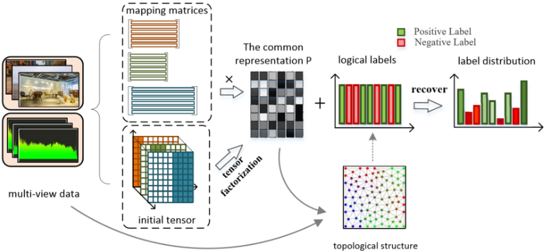
Label enhancement (LE) is a procedure of recovering the label distributions from the logical labels in the multi-label data, the purpose of which is to better represent and mine the label ambiguity problem through the form of label distribution. Existing LE work mainly concentrates on how to leverage the topological information of the feature space and the correlation among the labels, and all are based on single view data. In view of the fact that there are many multi-view data in real-world applications, which can provide richer semantic information from different perspectives, this paper first presents a multi-view label enhancement problem and proposes a tensor-based multi-view label enhancement method, named TMV-LE. Firstly, we introduce the tensor factorization to get the common subspace which contains the high-order relationships among different views. Secondly, we use the common representation and multiple views to jointly mine a more comprehensive topological structure in the dataset. Finally, the topological structure of the feature space is migrated to the label space to get the label distributions. Extensive comparative studies validate that the performance of multi-view multi-label learning can be improved significantly with TMV-LE.
- [Boutell et al., 2004] Matthew R. Boutell, Jiebo Luo, Xipeng Shen, and Christopher M. Brown. Learning multi-label scene classification. Pattern Recognition, 37(9):1757-1771, 2004.
- [Boyd et al., 2011] Stephen P. Boyd, Neal Parikh, Eric Chu, Borja Peleato, and Jonathan Eckstein. Distributed opti- mization and statistical learning via the alternating direc- tion method of multipliers. Foundations and Trends in Ma- chine Learning, 3(1):1-122, 2011.
- [Duygulu et al., 2002] Pinar Duygulu, Kobus Barnard, João F. G. de Freitas, and David A. Forsyth. Object recognition as machine translation: Learning a lexicon for a fixed im- age vocabulary. In Proceeding of European Conference on Computer Vision, pages 97-112, 2002.
- [Elisseeff and Weston, 2001] André Elisseeff and Jason We- ston. A kernel method for multi-labelled classification. In Proceeding of Conference on Neural Information Process- ing Systems, pages 681-687, 2001.
- [Everingham et al., 2010] Mark Everingham, Luc Van Gool, Christopher K. I. Williams, John M. Winn, and An- drew Zisserman. The pascal visual object classes (VOC) challenge. International Journal of Computer Vision, 88(2):303-338, 2010.
- [Gayar et al., 2006] Neamat El Gayar, Friedhelm Schwenker, and Günther Palm. A study of the ro- bustness of KNN classifiers trained using soft labels. In Proceeding of Artificial Neural Networks in Pattern Recognition, pages 67-80, 2006.
- [Geng, 2016] Xin Geng. Label distribution learning. IEEE Transactions on Knowledge and Data Engineering, 28(7):1734-1748, 2016.
- [Jia et al., 2019] Xiuyi Jia, Xiang Zheng, Weiwei Li, Changqing Zhang, and Zechao Li. Facial emotion distri- bution learning by exploiting low-rank label correlations locally. In Proceeding of Conference on Computer Vision and Pattern Recognition, pages 9841-9850, 2019.
- [Kolda and Bader, 2009] Tamara G. Kolda and Brett W. Bader. Tensor decompositions and applications. SIAM Review, 51(3):455-500, 2009.
- [Li et al., 2015] Yu-Kun Li, Min-Ling Zhang, and Xin Geng. Leveraging implicit relative labeling-importance informa- tion for effective multi-label learning. In Proceeding of International Conference on Data Mining, pages 251-260, 2015.
- [Liu et al., 2015] Meng Liu, Yong Luo, Dacheng Tao, Chao Xu, and Yonggang Wen. Low-rank multi-view learning in matrix completion for multi-label image classification. In Proceeding of AAAI Conference on Artificial Intelligence, pages 2778-2784, 2015.
- [Luo et al., 2013] Yong Luo, Dacheng Tao, Chang Xu, Chao Xu, Hong Liu, and Yonggang Wen. Multiview vector- valued manifold regularization for multilabel image clas- sification. IEEE Transactions on Neural Networks and Learning Systems, 24(5):709-722, 2013.
- [Read et al., 2011] Jesse Read, Bernhard Pfahringer, Geoff Holmes, and Eibe Frank. Classifier chains for multi-label classification. Machine Learning, 85(3):333-359, 2011.
- [Tibshirani, 1996] Robert Tibshirani. Regression shrinkage and selection via the lasso. Journal of the Royal Statistical Society, 58(1):267-288, 1996.
- [Tuia et al., 2011] Devis Tuia, Jochem Verrelst, Luis Alonso-Chorda, Fernando Pérez-Cruz, and Gustavo Camps-Valls. Multioutput support vector regression for remote sensing biophysical parameter estimation. IEEE Geoscience and Remote Sensing Letters, 8(4):804-808, 2011.
- [Xu et al., 2018] Ning Xu, An Tao, and Xin Geng. Label en- hancement for label distribution learning. In Proceeding of International Joint Conference on Artificial Intelligence, pages 2926-2932, 2018. IJCAI
- [Zhang and Zhou, 2007] Min-Ling Zhang and Zhi-Hua Zhou. ML-KNN: A lazy learning approach to multi-label learning. Pattern Recognition, 40(7):2038-2048, 2007.
- [Zhang and Zhou, 2014] Min-Ling Zhang and Zhi-Hua Zhou. A review on multi-label learning algorithms. IEEE Transactions on Knowledge and Data Engineering, 26(8):1819-1837, 2014.
- [Zhang et al., 2013] Tongtao Zhang, Rongrong Ji, Wei Liu, Dacheng Tao, and Gang Hua. Semi-supervised learning with manifold fitted graphs. In Proceeding of International Joint Conference on Artificial Intelligence, pages 1896- 1902, 2013. IJCAI
- [Zhang et al., 2018] Changqing Zhang, Ziwei Yu, Qinghua Hu, Pengfei Zhu, Xinwang Liu, and Xiaobo Wang. Latent semantic aware multi-view multi-label classification. In Proceeding of AAAI Conference on Artificial Intelligence, pages 4414-4421, 2018.
- [Zhou et al., 2020] Tao Zhou, Changqing Zhang, Chen Gong, Harish Bhaskar, and Jie Yang. Multiview la- tent space learning with feature redundancy minimiza- tion. IEEE Transactions on Cybernetics, 50(4):1655- 1668, 2020.
- [Zhu et al., 2016] Xiaofeng Zhu, Xuelong Li, and Shichao Zhang. Block-row sparse multiview multilabel learning for image classification. IEEE Transactions on Cybernet- ics, 46(2):450-461, 2016.
References were extracted automatically from the PDF and may contain errors.
Full text extracted automatically from the PDF; figures, tables and equations may differ. The PDF is the version of record.
1 Introduction
Multi-label learning (MLL) can address the label ambiguity problem by describing an instance with a set of labels. However, MLL cannot obtain the relative importance of each label to an instance, so Geng [2016] proposed a more general machine learning paradigm called label distribution learning
∗Corresponding author: Xiuyi Jia. This work is jointly supported by the National Key R&D Program of China (2018YFB1003902), the National Natural Science Foundation of China (61773208, 61906090), the Natural Science Foundation of Jiangsu Province (BK20170809, BK20191287), the Fundamental Research Funds for the Central Universities (30920021131), and the China Postdoctoral Science Foundation (2018M632304).
(LDL) to express the label intensities. In recent years, LDL has made a great progress, but it is still limited by the lack of datasets with label distributions, because 1) it is costly to examine and weigh the description degree of each label to a particular instance, and 2) the description degree of each label to the instance often has no objective quantitative criteria. Therefore, a new learning paradigm called label enhancement (LE) is proposed by Xu et al. [2018] to convert multi-label datasets consisting of logical labels into label distribution datasets.
Existing LE work mainly concentrates on how to leverage the topological information of the feature space and the correlation among the labels. However, all these studies are based on single view data. In many real-world applications, a lot of data exists in the form of multiple views. For example, in image classification, a natural scene image can often be represented by its visual features such as HSV color histogram, globe feature (Gist) and scale invariant feature transform (SIFT), meanwhile it can be annotated with multiple labels {water, tree, sky}. These different descriptions of the same object from different approaches or different perspectives constitute multiple views (multi-view) of the object. Each individual view cannot characterize different labels comprehensively since different views encode different properties of data. In other words, there is consistency and complementarity in multi-view data, which can provide more comprehensive and richer information for label enhancement. Hence, in this paper, we first present the multi-view label enhancement problem and propose a tensor-based multi-view label enhancement method (TMV-LE) for multi-label classification.
The main challenge of multi-view label enhancement is how to integrate the multiple types of heterogeneous information. A natural way is to perform LE on each view separately, and dispose the obtained label distributions with decision fusion. However, there is a lack of effective communication among different views in this way. Another smarter way is mapping each view into a low-rank common representation subspace which contains shared semantics. This way enhances communication among different views, but the method of linear mapping can only mine the low-order relationships in multi-view dataset, and cannot excavate the more complex high-order non-linear relationships. Therefore, it is hard to ensure that common semantic information is fully tapped. To solve the above problem, we not only reconstruct each view individually through the mapping matrix and lowrank common representation, but also mine shared information from the integrated multi-views. Specifically, we stack the isomorphically processed views to form a third-order tensor, and construct the mutual constraints of the factor matrices and the mapping matrices, which allows us to not only ensure the rationality of local single views, but also take advantage of the complementarity of global multiple views. By introducing the tensor, we can effectively enhance the potential communication among different views to obtain the more complex relationship. Finally, we jointly use the common representation and all original views to capture the more comprehensive topological structure in the dataset, then migrate it to the label space to reconstruct the label distribution. Because of the lack of multi-view label distribution datasets, we apply TMV-LE to multi-view multi-label classification tasks, and compare our proposed method with several state-of-theart multi-view multi-label learning approaches.
The main contributions of this paper are as follows: 1) We propose a novel label enhancement method TMV-LE, to our best knowledge, it is the first try to study label enhancement in the multi-view framework. 2) We propose a new method for constructing multi-view common representation. By introducing tensor factorization, the high-order relationships among different views can be mined.
2 RelatedWork
2.1 Multi-ViewMulti-Label Learning
Multi-label learning has been widely studied in recent years. Following [Zhang and Zhou, 2014], existing multi-label methods can be categorized into two groups, i.e, problem transformation methods and specialized algorithms. Problem transformation methods aim to decompose the problem into a series of binary classification problems. Such as Binary Relevance [Boutell et al., 2004] and ML-kNN [Zhang and Zhou, 2007]. Specialized algorithm methods tackle multilabel learning problem by designing specialized algorithms according to the characteristics of multi-label learning. Both ML-KM [Elisseeff and Weston, 2001] and ML-CC [Read et al., 2011] are specialized algorithms.
Multi-view learning can be embedded into multi-label learning naturally to further improve the classification performance by exploit a multi-view latent space [Zhou et al., 2020]. Recently, a few MVML classification methods [Luo et al., 2013] were proposed to exploit the complementarity of different types of features for the improved classification performance. Such as lrMMC [Liu et al., 2015] seeked a common low-dimensional representation under the matrix factorization framework and then conducts classification based on matrix completion. Zhang et al. [2018] tried to remain latent semantic when studying the low-dimensional common representation.
2.2 Label Enhancement
Label Enhancement (LE) aims at recovering the label distributions from the logical labels in the training set. Many LE algorithms have been proposed in recent years. Graph laplacian label enhancement (GLLE) [Xu et al., 2018] mines the hidden label importance from the training set via leveraging the topological information of the feature space. The LE algorithm based on label propagation (LP) [Li et al., 2015] recovers the label distributions from logical labels by using iterative label propagation technique. And the fuzzy clusteringbased LE algorithm (FCM) [Gayar et al., 2006] uses membership degree to determine the degree of which cluster each instance belongs to, and then converts it into the membership of each label by fuzzy composition. To the best of our knowledge, there are currently no related work reports on multiview label enhancement.
3 Notation and Background
We first introduce some related concepts and notations of tensors used throughout of the paper. More details about tensor algebra, please refer to [Kolda and Bader, 2009]. The order of a tensor is the number of dimensions, also known as modes. An M-th order tensor is represented as X ∈ RI1×···×IM , where IM is the cardinality of its IM-th mode.
Definition 1 (Rank-One Tensors). An M-way tensor X ∈ RI1×···×IM is rank-one if it can be written as the outer product of M vectors, i.e.,X = a(1) ◦ a(2) ◦ · · ·a(M) , (1)
the symbol "◦" represents the vector outer product. This means that each element of the tensor is the product of the corresponding vector elements:
Definition 2 (CP Factorization). Given an M-th order tensor X ∈ RI1×···×IM , the CP factorization is defined by factor matrices A(m) ∈ RIm×r for m = 1, 2, ...,M, respectively, such that
where r is the rank of the tensor X, defined as the smallest number of rank-one tensors in an exact CP factorization. The factor matrices A(1) , A(2) , ..., A(M) can be viewed as the common latent feature matrices in different modes.
4 Methodology
Given a multi-view dataset consisting of n instances with V views that are denoted as a set of feature matrices X = {X(v) ∈ Rn×dv }Vv=1 , where dv is the dimension of the v-th view. And the label space is Y = [y1, y2, ..., yn] ∈ {0, 1}n×l , where l is the number of labels. We use both the matrix factorization framework and CP factorization to decompose a lowrank common representation matrix P from all views. Then, we design the LE algorithm with the topological structure from the common representation and all views. The whole framework of TMV-LE is shown in Figure 1.
4.1 Construct Common Representation
To find a low-rank common representation P, the traditional distributed strategy is adopted to optimize the following problem [Liu et al., 2015; Zhang et al., 2018]:
where P ∈ Rn×r is the low-rank common representation. Since the rank of a matrix is difficult to optimize, the trace norm ‖.‖tr is utilized as a convex approximation of the rank of a matrix. B(v) ∈ Rdv×r is the mapping matrix of v-th view. Each X(v) can be reconstructed using B(v) and P . But in this framework, the mapping process of different views is completely independent, which makes it difficult for the common representations to obtain complete shared information. So we introduce tensor to enhance the communication between different views during the mapping process.
First, we need to construct an initial tensor. In order to eliminate the heterogeneity between different views, that is, the feature dimensions of different views are different. we propose an isomorphism approach. Specifically, each view is extended to a n × ds matrix, where ds = ∑Vv=1 dv, and the expanded views are stacked to form a tensor X. Each feature matrix is arranged diagonally in the third-order tensor. And in the following method, we will replace the original views with expanded views. This isomorphism approach can do not only completely retain the information of all views, but also reflect the sequence relationship between views. It is worth mentioning that how to assign extended features on each view will have a great impact on the entire model. A simple way is to take 0, but this will cause the entire tensor to be sparse, and assigning 0 to unknown data is also not a realistic choice. So we introduce a tensor completion method. A nonnegative weight tensor W, which has the same size as X, is constructed as:
We focus on using a weighted version of the error function to ignore extended features and model the original views only. As mentioned above, the CP factorization model is applied to get the common factor matrices across all the views. The weighted version is
where X ∈ Rn×ds×V , B∗ ∈ Rds×r and H ∈ RV×r , "◦" is the Hadamard product, i.e. the elementwise matrix product. Eq. (4) and Eq. (6) contain the same common representation P to jointly mine shared semantic from multiple views. As mentioned above, the tensor we constructed can well reflect the sequence relationship among views, while the factor matrix H is the combination of the rank-one components on the axis of views' sequence. So H needs to identify different views as an indicator matrix. In other words, H should contain only the information that distinguishes different views but not the specific information about different feature views. Therefore, we add the l2,1-regularization on H to make it row-sparse.
According to [Kolda and Bader, 2009], CP factorization can be written in the following matricized form:
where X(1) is the mode-1 matricization of X, ⊙ denotes Khatri-Rao product. Meanwhile, according to Eq. (4), our initial tensor also can be written as a representation consisting of {P(B(v) )T }Vv=1 . H is the indicator matrix with no feature information, so the difference between B∗ and each mapping matrix B(v) should not be too large. At the same time, in order to better explore the complementarity between different views, we learn a non-negative weight parameter θv for each view v. The larger the weight θv, the more the v-th view should ensure that the mapping matrix B(v) is similar to B∗ . After explaining all the factor matrices and applying the corresponding constraints, the final objective function is as follows:
where λ1, λ2, λ3, λ4 are trade-off parameters. By optimizing Eq. (8), we can obtain the low-rank common representation P from multiple views, and then we use LE for multi-label classification.
4.2 Label Enhancement
In LE, the information of the feature space and the logical label space are usually used to reconstruct the numerical labels of each instance. Thus we assume that the feature space and the label space are linearly related, and we get the following loss terms:
where D = PW + b, P is the common representation obtained in the above, D is the predicted label distributions, W is the weight matrix, and b is a bias vector.
Considering that the common representation is a low-rank space, we introduce Local Linear Embedding (LLE) [Tuia et al., 2011] and the smoothness assumption [Zhang et al., 2013] into our method. Specifically, each point can be reconstructed by a linear combination of its neighbors, at the same time, the numerical label space and the feature space should share similar local topological structure. We use the common representation and multiple views to jointly mine a more comprehensive topological structure in the dataset. The approximation of the topological structure of the feature space can be obtained by solving the following problem:
where Mij represents the weight of the relationship between instance i and instance j, and Mij = 0 if Pj is not one of Pi's K-nearest neighbors. ∑ni=1 Mij is constrained because of the translation invariance. θv is the parameter to measure the complementarity between different views that was learned in Eq. (8). In order to make the topological structure more flexible, we use this weight parameter in Eq. (10). By solving Eq. (10), we obtain the weight matrix M, and then migrate the topological structure of the feature space to the label space by using Eq. (11):
In addition, considering there may be correlations among different labels, i.e., some labels often appear together while some often conflict to each other, we introduce the label correlations into our LE method.
In real-world applications, label correlations are usually local, where a label correlation may be shared by only a subset of instances rather than all instances. So we adopt a low-rank structure to implicitly exploit the label correlations at the local level [Jia et al., 2019]. The training set is divided into k clusters and each cluster has a low-rank structure,
Combining Eq. (9), Eq. (11) and Eq. (12), the LE framework can be rewritten as:
where α, β are trade-off parameters. In order to distinguish the relevant and irrelevant labels, we add an extra virtual label in the training set, which represents the threshold of distinguishing the relevant and the irrelevant labels. Since 1 or 0 is used in multi-label data to indicate whether the label is relevant to the example or not, we initialize the virtual label to 0.5 and train the corresponding parameters for the virtual label. At the prediction stage, given a test instance, the predicted numerical label greater than the predicted virtual label is relevant to the example, and vice versa.
4.3 Optimization Framework
ADMM (Alternating Direction Method of Multipliers) [Boyd et al., 2011] which is suitable for addressing those objective functions with linear constraints, is proper for solving Eq. (8) and Eq. (13).
Eq. (8) can be solved by the following alternative methods in iteration t:
where C = H⊙B∗ , E = H⊙P , F = B∗⊙P , Z = P , Ws is the W spread out on mode-s, Λ1 is the Lagrange multipliers, q, ρ1 are penalty parameters and < ·, · > is the Frobenius dotproduct. Eq. (14), Eq. (15), Eq. (16), Eq. (17), and Eq. (18) can be solved by the limited memory quasi-Newton method (L-BFGS), due to the page limitation, we do not describe the details of the solution of every sub-problem. Eq. (19) has closed-form solution according to [Tibshirani, 1996], and can be solved by the following Lemma 1:
Lemma 1 For matrix Y ∈ Rn×d and µ > 0, the problem as follows has the only one analysis solution,
This solution can be described by singular value thresholding operator,
U ∈ Rn×r , V ∈ Rd×r and σ = {σ1, σ2, · · · , σr} ∈ Rr×1 can be achieved by singular decomposition of matrix Y , Y = UΣV T and Σ = diag(σ).
Eq. (13) can be solved by the following alternative methods in iteration t:
| Dataset | Emotions | Yeast | Corel5k | PASCAL VOC |
|---|---|---|---|---|
| #Instances | 593 | 2417 | 4999 | 9963 |
| #Views | 2 | 2 | 3 | 3 |
| #Features | 8 / 64 | 24 / 79 | 100 / 512 / 1000 | 100 / 512 / 1000 |
| #Labels | 6 | 14 | 260 | 20 |
where Λ2 is the Lagrange multipliers, ρ2 is penalty parameter and Q(i) = D(i) . Eq. (21) can be solved by L-BFGS. Similar to Eq. (19), we get the closed-form solution of Eq. (22) according to Lemma 1.
5 Experiments
5.1 Datasets &Features
In this section, we implement our experiments on four realworld MVML datasets. Yeast is a biological experiments dataset, it has two views including the concatenation of the genetic expression (79 attributes) and the phylogenetic profile of a gene (24 attributes). Emotions is a music emotion experiments dataset, it has two views including rhythmic (8 attributes) and timbre (64 attributes). Corel5k [Duygulu et al., 2002] and PASCAL VOC [Everingham et al., 2010] are two image recognition datasets. There are three types of features, i.e., two types of local features: DenseHue and DenseSift and one type of global features: Gist, where each type of features can be regarded as one view. The dimensionalities of DenseHue, DenseSift and Gist are 100, 1000 and 512, respectively. Some basic statistics about these four datasets are given in Table 1.
5.2 Comparing Algorithms &EvaluationMetrics
Since this is the first time to propose LE in the multi-view framework, in order to verify the effectiveness of our proposed method, we apply TMV-LE to multi-view multi-label classification task, and compare with several existing multiviewmulti-label algorithms.
The TMV-LE algorithm is compared with five algorithms, including three MVML algorithms lrMMC, LSA-MML and F2L21F [Zhu et al., 2016], a multi-label algorithmML-kNN with two types of feature inputs. ML-kNN(C) means the input to ML-KNN is the concatenation of all views, and ML-kNN(B) means input is the view with best performance. We use the suggested parameters reported in corresponding literature. For ML-kNN(B) and ML-kNN(C), the parameter k is set to 10. In F2L21F, the parameters λ1 and λ2
| Dataset | Metric | MVML methods | LE methods | |||||||
|---|---|---|---|---|---|---|---|---|---|---|
| TMV-LE | ML-kNN(B) | ML-kNN(C) | LSA-MML | F2L21F | lrMMC | MV-LE | GLLE-C | GLLE-L | ||
| Ham-Loss↓ | 0.158±0.006 | 0.200±0.016• | 0.193±0.012• | 0.284±0.019• | 0.225±0.024• | 0.262±0.020• | 0.173±0.010• | 0.221±0.012• | 0.218±0.011• | |
| Emotions Coverage↓ | 0.286±0.021 | 0.303±0.021• | 0.299±0.021 | 0.315±0.030• | 0.301±0.024 | 0.338±0.030• | 0.301±0.023 | 0.310±0.025• | 0.302±0.020 | |
| Ave-Pre↑ | 0.818±0.007 | 0.795±0.020• | 0.799±0.032 | 0.779±0.040• | 0.798±0.030 | 0.772±0.033• | 0.799±0.013• | 0.783±0.022• | 0.792±0.019• | |
| Micro-F1↑ | 0.742±0.010 | 0.652±0.030• | 0.668±0.026• | 0.185±0.067• | 0.651±0.038• | 0.662±0.035• | 0.672±0.018• | 0.651±0.036• | 0.662±0.033• | |
| Ham-Loss↓ | 0.158±0.004 | 0.208±0.008• | 0.195±0.009• | 0.298±0.005• | 0.315±0.012• | 0.286±0.008• | 0.184±0.006• | 0.205±0.006• | 0.192±0.004• | |
| Yeast Coverage↓ | 0.442±0.012 | 0.455±0.008• | 0.450±0.012 | 0.623±0.011• | 0.627±0.011• | 0.625±0.014• | 0.448±0.012 | 0.459±0.011• | 0.455±0.013• | |
| Ave-Pre↑ Micro-F1↑ | 0.812±0.006 0.739±0.007 | 0.753±0.009• 0.608±0.013• | 0.764±0.012• 0.639±0.016• | 0.611±0.013• 0.035±0.008• | 0.607±0.016• 0.465±0.020 • | 0.608±0.013• 0.565±0.018• | 0.770±0.009• 0.651±0.010• | 0.743±0.012• 0.614±0.010• | 0.751±0.012• 0.626±0.011• | |
| Ham-Loss↓ | 0.012±0.000 | 0.012±0.000 | 0.012±0.000 | 0.013±0.000• | 0.017±0.000• | 0.014±0.001• | 0.013±0.001 | 0.014±0.000• | 0.014±0.000• | |
| Corel5k Coverage↓ | 0.258±0.010 | 0.262±0.014 | 0.249±0.013 | 0.327±0.013• | 0.559±0.020• | 0.502±0.016• | 0.262±0.011 | 0.267±0.012 | 0.265±0.011 | |
| Ave-Pre↑ | 0.553±0.000 | 0.416±0.009• | 0.441±0.010• | 0.475±0.014• | 0.314±0.013• | 0.452±0.013• | 0.464±0.005• | 0.439±0.009• | 0.446±0.008• | |
| Micro-F1↑ | 0.356±0.004 | 0.226±0.013• | 0.259±0.011• | 0.146±0.014• | 0.278±0.014• | 0.205±0.014• | 0.276±0.008• | 0.246±0.012• | 0.258±0.014• | |
| Ham-Loss↓ | 0.067±0.001 | 0.055±0.001◦ | 0.064±0.002◦ | 0.064±0.001◦ | 0.091±0.004• | 0.069±0.001• | 0.070±0.001• | 0.071±0.001• | 0.069±0.001• | |
| PASCAL Coverage↓ | 0.193±0.011 | 0.222±0.006• | 0.233±0.008• | 0.202±0.010 | 0.240±0.022• | 0.256±0.013• | 0.219±0.008• | 0.230±0.007• | 0.227±0.009• | |
| Ave-Pre↑ | 0.738±0.011 | 0.658±0.011• | 0.571±0.009• | 0.690±0.012• | 0.644±0.019• | 0.563±0.002• | 0.684±0.009• | 0.624±0.010• | 0.639±0.012• | |
| Micro-F1↑ | 0.482±0.012 | 0.447±0.019• | 0.327±0.019• | 0.259±0.013• | 0.471±0.017 | 0.251±0.017• | 0.462±0.013• | 0.404±0.015• | 0.422±0.014• | |
are both set 10. For LSA-MML, the parameter r is chosen among {2, 3, 4, 5}, the parameters α and β are chosen among {0.01, 0.1, 1, 10, 100}. In lrMMC, the parameter µ is determined as in MC-1, and the parameter γ is tuned over the set {10i |i = -4,-3, ..., 3}. For TMV-LE, the parameters {λi|i = 1, 2, 3, 4}, α and β are chosen among {0.01, 0.1, 1, 10, 100}, the parameter k is set to 10. And the clustering method used in TMV-LE is spectral clustering.
In addition, we select three comparing algorithms to distinguish the different roles of tensor factorization and LE framework. In order to verify that our method of constructing the common representation has an effect on the experimental results, in MV-LE, we adopt the method of constructing the common representation in Eq. (4), and then use our proposed LE method to perform label enhancement and classification. We also modify a popular LE method GLLE to adapt the multi-view datasets, named GLLE-C and GLLE-L, respectively. In GLLE-C, we use the concatenation of all views as the input. In GLLE-L, we make a decision fusion of the results on different views. Specifically, we add the weights of different views during the training process, and finally use the weights to fuse multiple results. For GLLE, the parameter λ is chosen among {0.01, 0.1, ..., 100}, and the number of neighbors K is set to c + 1, c is the number of labels. The kernel function in GLLE is Gaussian kernel.
Due to page limitation, we just choose four evaluation metrics that mostly used for multi-label classification, including Hamming Loss(Ham-Loss), Coverage, Average Precision(Ave-Pre) and Micro-F1, which consider the performance of multi-label predictor from various aspects. The former 2 measures are smaller the better and the latter 2 measures are larger the better. For each dataset, ten-fold crossvalidation is performed where the mean results and standard deviations are recorded for all comparing algorithms.
5.3 Experimental Results
ComparisonwithMVMLmethods. Table 2 demonstrates the classification comparison of different methods on four datasets. The two-tailed t-tests at the 5% significance level are performed. By analyzing the experimental results, we can obtain the following two conclusions: 1) Among the 16 configurations (4 datasets × 4 evaluation metrics), TMV-LE ranks 1st in 81.3% cases respectively. In a big picture, our algorithm almost achieves the best performance on all datasets, which clearly demonstrates the advantages of our method in exploring MVML data. 2) It is clear that for the traditional single-view multi-label method, the performance of the view concatenating strategy is always better than the best single view. This verifies the effectiveness of multi-view learning compared to single-view learning, as the complementarity among different views is very important.
Comparison with LE methods. From Table 2, we can draw the following conclusions: 1) The tensor-based common representation construction method we proposed is effective, because compared with MV-LE, TMV-LE achieves a significantly better result, while both TMV-LE and MV-LE applied the same LE method; 2) The LE method we proposed is effective, because MV-LE is better than most MVML methods, and MV-LE only uses a very simple method to construct a common representation. 3) Both GLLE-C and GLLE-L adopt the multi-view datasets, however, their results are almost all worse than that of TMV-LE and MV-LE, which also indicates the effectiveness of our proposal.
6 Conclusions
In this paper, we first propose a novel two-stage multi-view label enhancement algorithm TMV-LE. By constructing the mutual constraint between tensor factorization and mapping matrices, we mine the high-order relationships among multiple views. Then, we use multiple views to more comprehensively mine the topological structure in the feature space and migrate it to the label space to obtain the label distribution. The experimental results on several datasets demonstrate the superiority of TMV-LE on multi-view multi-label tasks.
@inproceedings{ijcai2020p328,
  title     = {Tensor-based multi-view label enhancement for multi-label learning},
  author    = {Zhang, Fangwen and Jia, Xiuyi and Li, Weiwei},
  booktitle = {Proceedings of the Twenty-Ninth International Joint Conference on
               Artificial Intelligence, {IJCAI-20}},
  publisher = {International Joint Conferences on Artificial Intelligence Organization},
  editor    = {Christian Bessiere},
  pages     = {2369--2375},
  year      = {2020},
  month     = {7},
  note      = {Main track},
  doi       = {10.24963/ijcai.2020/328},
  url       = {https://doi.org/10.24963/ijcai.2020/328},
}
TY - CPAPER TI - Tensor-based multi-view label enhancement for multi-label learning AU - Zhang, Fangwen AU - Jia, Xiuyi AU - Li, Weiwei T2 - Proceedings of the Twenty-Ninth International Joint Conference on Artificial Intelligence, IJCAI-20 PB - International Joint Conferences on Artificial Intelligence Organization PY - 2020 SP - 2369 EP - 2375 DO - 10.24963/ijcai.2020/328 UR - https://doi.org/10.24963/ijcai.2020/328 ER -Copied
Machine-readable versions of this paper, for tools and AI agents:





