
Semi-Supervised Learning with Manifold Fitted Graphs
Proceedings of the Twenty-Third International Joint Conference on Artificial Intelligence. Pages 1896-1901.
© 2013 International Joint Conferences on Artificial Intelligence
Abstract
In this paper, we propose a locality-constrained and sparsity-encouraged manifold fitting approach, aiming at capturing the locally sparse manifold structure into neighborhood graph construction by exploiting a principled optimization model. The proposed model formulates neighborhood graph construction as a sparse coding problem with the locality constraint, therefore achieving simultaneous neighbor selection and edge weight optimization. The core idea underlying our model is to perform a sparse manifold fitting task for each data point so that close-by points lying on the same local manifold are automatically chosen to connect and meanwhile the connection weights are acquired by simple geometric reconstruction. We term the novel neighborhood graph generated by our proposed optimization model M-Fitted Graph since such a graph stems from sparse manifold fitting. To evaluate the robustness and effectiveness ofM -fitted graphs, we leverage graph-based semisupervised learning as the testbed. Extensive experiments carried out on six benchmark datasets validate that the proposed M -fitted graph is superior to state-of-the-art neighborhood graphs in terms of classification accuracy using popular graph-based semi-supervised learning methods.
- [Belkin and Niyogi, 2003] M. Belkin and P. Niyogi. Laplacian eigenmaps for dimensionality reduction and data representa- tion. Neural Computation, 15(6):1373-1396, 2003.
- [Belkin et al., 2006] M. Belkin, P. Niyogi, and V. Sindhwani. Manifold regularization: a geometric framework for learn- ing from labeled and unlabeled examples. Journal of Ma- chine Learning Research, 7:2399-2434, 2006.
- [Bohanec and Rajkovič, 1988] M. Bohanec and V. Rajkovič. Knowledge acquisition and explanation for multi-attribute decision. In Proc. International Workshop of Expert Systems and Their Applications, 1988.
- [Breiman et al., 1984] L. Breiman, J. H. Friedman, R. A. Ol- shen, and C. J. Stone. Classification and Regression Trees. Statistics/Probability Series. Wadsworth Publishing Com- pany, Belmont, California, U.S.A., 1984.
- [Candés and Tao, 2005] E. Candés and T. Tao. Decoding by linear programming. IEEE Transactions on Information Theory, 51(12):4203-4215, 2005.
- [Cheng et al., 2009] H. Cheng, Z. Liu, and J. Yang. Sparsity induced similarity measure for label propagation. In Proc. ICCV, 2009.
- [Elhamifar and Vidal, 2009] E. Elhamifar and R. Vidal. Sparse subspace clustering. In Proc. CVPR, 2009.
- [Elhamifar and Vidal, 2010] E. Elhamifar and R. Vidal. Clus- tering disjoint subspaces via sparse representation. In Proc. International Conference on Acoustics, Speech, and Signal Processing, 2010.
- [Elhamifar and Vidal, 2011] E. Elhamifar and R. Vidal. Sparse manifold clustering and embedding. In NIPS 24, 2011.
- [Frank and Asuncion, 2010] A. Frank and A. Asuncion. UCI machine learning repository, 2010.
- [Gao et al., 2010] S. Gao, I. W. Tsang, and L. Chia. Ker- nel sparse representation for image classification and face recognition. In Proc. ECCV, 2010.
- [Hastie et al., 2009] T. Hastie, R. Tibshirani, and J. H. Fried- man. The elements of statistical learning: data mining, inference, and prediction. Second Edition, New York: Springer-Verlag, 2009.
- [Jebara et al., 2009] T. Jebara, J. Wang, and S.-F. Chang. Graph construction and b-matching for semi-supervised learning. In Proc. ICML, 2009.
- [Jiang et al., 2012] Y.-G. Jiang, Q. Dai, J. Wang, C.-W. Ngo, X. Xue, and S.-F. Chang. Fast semantic diffusion for large- scale context-based image and video annotation. IEEE Transactions on Image Processing, 21(6):3080-3091, 2012.
- [Jing and Baluja, 2008] Y. Jing and S. Baluja. Visualrank: Applying pagerank to large-scale image search. IEEE Transactions on Pattern Analysis and Machine Intelligence, 30(11):1877-1890, 2008.
- [Liu and Chang, 2009] W. Liu and S.-F. Chang. Robust multi- class transductive learning with graphs. In Proc. CVPR, 2009.
- [Liu et al., 2010] W. Liu, J. He, and S.-F. Chang. Large graph construction for scalable semi-supervised learning. In Proc. ICML, 2010.
- [Liu et al., 2011a] W. Liu, Y.-G. Jiang, J. Luo, and S.-F. Chang. Noise resistant graph ranking for improved web im- age search. In Proc. CVPR, 2011.
- [Liu et al., 2011b] W. Liu, J. Wang, S. Kumar, and S.-F. Chang. Hashing with graphs. In Proc. ICML, 2011.
- [Nene et al., 1996] S. A. Nene, S. K. Nayar, and H. Murase. Columbia Object Image Library (COIL-20). Technical re- port, Columbia University, 1996.
- [Ng et al., 2001] A. Y. Ng, M. I. Jordan, and Y. Weiss. On spectral clustering: Analysis and an algorithm. In NIPS 14, 2001.
- [van Breukelen and Duin, 1998] M. van Breukelen and R. P. W. Duin. Neural network initialization by combined classifiers. In Proc. International Conference on Pattern Recognition, 1998.
- [Wang and Zhang, 2008] F. Wang and C. Zhang. Label propa- gation through linear neighborhoods. IEEE Transactions on Knowledge and Data Engineering, 20(1):55-67, 2008.
- [Weston et al., 2003] J. Weston, C. S. Leslie, D. Zhou, A. Elis- seeff, and W. S. Noble. Semi-supervised protein classifica- tion using cluster kernels. In NIPS 16, 2003.
- [Xu et al., 2011] B. Xu, J. Bu, C. Chen, D. Cai, X. He, W. Liu, and J. Luo. Efficient manifold ranking for image retrieval. In Proc. SIGIR, 2011.
- [Zhang and Zha, 2004] Z. Zhang and H. Zha. Principal man- ifolds and nonlinear dimensionality reduction via tangent space alignment. SIAM Journal on Scientific Computing, 26(1):313-338, 2004.
- [Zhang, 2011] T. Zhang. Adaptive forward-backward greedy algorithm for learning sparse representations. IEEE Trans- actions on Information Theory, 57(7):4689-4708, 2011.
- [Zhou et al., 2003a] D. Zhou, O. Bousquet, T. N. Lal, J. We- ston, and B. Schölkopf. Learning with local and global con- sistency. In NIPS 16, 2003.
- [Zhou et al., 2003b] D. Zhou, J. Weston, A. Gretton, O. Bous- quet, and B. Schölkopf. Ranking on data manifolds. In NIPS 16, 2003.
- [Zhu and Goldberg, 2009] X. Zhu and A. B. Goldberg. Intro- duction to Semi-Supervised Learning. Morgan & Claypool, 2009.
- [Zhu et al., 2003] X. Zhu, Z. Ghahramani, and J. D. Lafferty. Semi-supervised learning using gaussian fields and har- monic functions. In Proc. ICML, 2003.
References were extracted automatically from the PDF and may contain errors.
Full text extracted automatically from the PDF; figures, tables and equations may differ. The PDF is the version of record.
1 Introduction
In this paper, we investigate the problem of Graph-Based Semi-Supervised Learning [Zhu and Goldberg, 2009] which is an emerging machine learning topic having received broad research attention and also triggered a variety of practical applications including document and image ranking [Zhou et al., 2003b], web-scale image search [Jing and Baluja, 2008][Liu et al., 2011a], image and video annotation [Jiang et al., 2012], protein classification [Weston et al., 2003], etc. To accomplish sensible semi-supervised learning, the key challenge arises, i.e., how to build a robust neighborhood graph which is capable of capturing the inherent manifold structure underlying input data samples. After constructing such a Wei Liu♮
♮ IBM Research, USA weiliu@us.ibm.com
Gang Hua♮♯
♯Stevens Inst. of Technology, USA
ghua@stevens.edu
graph, representative semi-supervised learning methods, e.g., [Zhu et al., 2003][Zhou et al., 2003a][Belkin et al., 2006][Liu and Chang, 2009], can be readily deployed through engaging this graph in proper smoothness regularization terms. A typical kind of graphs are kNN graphs which have been intensively used in a number of learning problems such as dimensionality reduction [Belkin and Niyogi, 2003] and spectral clustering [Ng et al., 2001] besides semi-supervised learning studied in this paper. To construct a kNN graph on an input dataset X = {x1, · · · , xn} ⊂ Rd with cardinality |X| = n, edges are established to connect each individual data point and its k nearest neighbors. The edge weights are then obtained by either parametric kernel functions (typically the Gaussian kernel) or nonparametric optimization procedures [Jebara et al., 2009]. However, kNN graphs do not explicitly explore or capture intrinsically low-dimensional manifolds on which high-dimensional data samples reside, though they can approximate some manifolds existing in simple datasets.
Towards capturing geometric structure hidden in data into graph construction mechanisms, one recent trend is to explore the sparse subspace structure [Elhamifar and Vidal, 2009][Elhamifar and Vidal, 2010][Elhamifar and Vidal, 2011][Gao et al., 2010], which has turned out to be very effective for discovering the clusters formed in high-dimensional data such as face images. Specifically, [Elhamifar and Vidal, 2009][Elhamifar and Vidal, 2010] proposed to reconstruct each individual data point xi using the rest of points in X in a least squares sense. Very importantly, for each instance xi a sparsity constraint is imposed to make such a geometric reconstruction find the most fitted subspace spanned by a few instances in X. In another words, the found subspace holds the shortest distance to the point xi meanwhile keeping the subspace dimension as low as possible. This sparse subspace fitting problem can be relaxed to an ℓ1 minimization problem [Cand´es and Tao, 2005] and thus solved by conventional convex optimization techniques. In addition, the seminal work [Gao et al., 2010] and [Elhamifar and Vidal, 2011] suggested similar geometric reconstruction schemes in kernel-induced feature spaces and on manifolds, respectively. In the work, the sparsity constraint is enforced as well.
The key computational challenge of the aforementioned sparse subspace fitting scheme [Elhamifar and Vidal, 2009]
and its variants is that they require all, or at least a part, of the input dataset X to reconstruct every data point xi, that is, minimizing an ℓ1 problem (‖ · ‖1 denotes ℓ1 norm) of n - 1 variables
In reconstructing xi, this ℓ1 problem involves a basis X¯i = [x1, · · · , xi-1, xi+1, · · · , xn] that is composed of n - 1 instances in X except the target instance xi. Above all, the convex relaxation from ℓ0 norm to ℓ1 norm cannot guarantee that the resulting solution ai (i.e., the subspace reconstruction coefficient vector) is always meaningful. The ℓ1 minimization may lead to a dense ai and thus violate the sparsity expectation of the subspace reconstruction coefficients. Second, solving the ℓ1 problem in eq. (1) is nontrivial and timeconsuming for high-dimensional or large-scale data. Third, the sparse subspace fitting scheme neglects the locality of data and is hence likely to introduce irrelevant instances that are outliers or from other classes with respect to xi. Finally and most critically, sparse subspace fitting assumes that a multi-subspace structure exists in the data, which is not always true for real-world data. It is noted that [Cheng et al., 2009] considered the locality constraint when performing sparse subspace fitting for neighborhood graph construction, but it still adopted the multi-subspace assumption.
In this paper, we argue that a multi-manifold structure is more natural than the multi-subspace structure for realistic datasets. The latter can be regarded as an extreme case of the multi-manifold structure.
In order to overcome the potential issues associated with sparse subspace fitting, in this work we propose a locality-constrained and sparsity-encouraged reconstruction approach, namely Sparse Manifold Fitting, which can capture the locally sparse manifold structure and thus discover the global multi-manifold structure. The proposed approach yields a novel neighborhood graph called by M-Fitted Graph. In sparse manifold fitting, we directly design an ℓ0 norm-based optimization model to perform sparse coding with the locality constraint that restricts the coding within the scope of a limited number of neighbors, thereby ensuring the optimization efficiency.
Our M-fitted graphs can benefit vast applications which previously used kNN graphs. To validate the robustness and effectiveness of M-fitted graphs, we adopt graph-based semisupervised learning as the testbed since its classification accuracy heavily depends on the quality of used graphs. Through extensive experiments, we find that our M-fitted graphs are very suitable for semi-supervised learning and exhibit superior performance over state-of-the-art neighborhood graphs when cooperating with representative semi-supervised learning techniques, e.g., Local and Global Consistency (LGC) [Zhou et al., 2003a], Linear Neighborhood Propagation (LNP) [Wang and Zhang, 2008], and Gaussian Fields and Harmonic Functions (GFHF) [Zhu et al., 2003].
The remainder of this paper is organized as follows: we first introduce M-fitted graphs, subsequently present the sparse manifold fitting approach for constructing M-fitted graphs, then illustrate the usage in the context of graph-based semi-supervised learning, and finally show the quantitative experimental results.
2 M-Fitted Graphs
Notations. We define the input data matrix as X = [x1, . . . , xn] ⊂ Rd×n of d feature dimensions and n instances. We formulate the neighborhood graph to be constructed as an affinity matrix W ∈ Rn×n where wij represents the edge weight between vertices xi and xj. We define by M the manifold(s) underlying the input dataset X, {Ti}ni=1 the local tangent spaces, {Ui}ni=1 the local direction basis matrices, and {Fi}ni=1 the local affine subspaces.
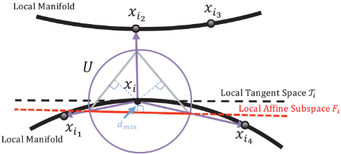
Geometric Idea. Following the well-known manifold learning approach Local Tangent Space Alignment [Zhang and Zha, 2004], we assume that the manifold(s) (possibly multiple manifolds) underlying the input data collection X are composed of and merged by a series of local tangent spaces. Each tangent space, denoted by Ti, lies under each data point xi. In mathematics, we can writeM= ⋃ni=1 Ti if n →∞, where a local tangent space Ti is actually a small patch of a local manifold fromM. Then our goal is to seek such a tangent space located at each point. We employ the geometric sparsity idea proposed in [Elhamifar and Vidal, 2011] to approximately seek the local tangent spaces. Specifically, we reconstruct each data point xi using sparse bases from a local direction basis Ui, and the minimal reconstruction distortion is pursued to yield the optimal local directions that determine the optimally fitted local affine subspace Fi for xi. As a result, this sparse reconstruction gives rise to the local affine subspace Fi with the minimal angle to the target local tangent space Ti, therefore discovering the best fitted local manifold.
Through sparse reconstruction, we can build a neighborhood graph in which the graph edges correspond to the solved local directions. Under such a circumstance, the edges connecting to xi are closely parallel to the local tangent space Ti and thus closely reside on the local manifold at xi.
Formulation. Our proposed sparse reconstruction starts from setting up a relatively large neighborhood of m (m < n) neighbors (record xi's neighbor indices into [i1, ..., im]), and then eliminates the unqualified ones.
We normalize the difference vectors between xi and its m neighbors to remove distance variations while preserving structural cues, and then form a local direction basis matrix
Now, our task is to find the local affine subspace Fi that fits xi as much as possible. As intuitively illustrated in Fig. 1, we pursue the minimal distance between xi and the ambient affine subspace
That is, min1⊤ci=1 ‖xi - xi -Uici‖ = ‖Uici‖. Critically, a sparsity constraint ‖ci‖0 ≤ s (s < m) is imposed to reduce the risk of introducing outliers. In doing so, the nonzero elements in the reconstruction coefficient vector ci automatically select sparse local directions fromUi to generate a feasible local affine subspace. So far, we formulate the sparse reconstruction task as follows
whose core idea is to seek the best fitted local affine subspace Fi subject to the affine and sparsity constraints on the coefficient vector ci. Fig. 1 displays that the local affine subspace holding the minimal distance to the point xi also holds the minimal angle to the local tangent space Ti.
Graph Construction. The next step is to translate the coefficient vectors {ci}ni=1 , solved in sparse reconstruction, into the graph edge weights {wij}ni,j=1 . Let ci = [c1i, · · · , cmi]⊤. For each vertex (i.e., data point) xi, we obtain the edge weights wij ,i's via re-normalizing cji's:
It is worth mentioning that although we eliminate the distance information in eq. (2), we take it back in eq. (5) to make the neighbors closer to xi contribute larger edge weights.
Like [Cheng et al., 2009], we deal with the negative weights as follows
where wi is the i-th column vector of the graph affinity matrix W. Finally, we conduct a symmetrizing step
We term the graph of the affinity matrix WM-Fitted Graph, which is yielded through the sparse reconstruction in eq. (4) and the graph construction steps in eqs. (5)(6)(7).
In contrast to Sparse Manifold Clustering and Embedding (SMCE) [Elhamifar and Vidal, 2011], our proposedMfitted graph not only eliminates the incorrect edges connecting points not lying on the same local manifold, but also keeps the sparse edge connections. The sparsity originates from directly solving an ℓ0 problem (see Section 3) instead of the ℓ1 problem in [Elhamifar and Vidal, 2011]. Note that in SMCE the edges connecting to some outliers are tolerable, as SMCE is designed for clustering which is somewhat insensitive to the sparsity level of the graph affinity matrixW. However, in the scenario of graph-based semi-supervised learning, erroneous edge connections are unacceptable, so we discard negative reconstruction coefficients and enforce explicit sparsity (via ℓ0 norm) in producingW.
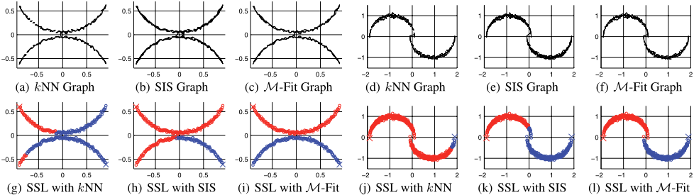
Fig. 2 visualizes the semi-supervised learning results produced by kNN graphs, Sparsity Induced Similarity (SIS) graphs [Cheng et al., 2009], andM-fitted graphs on two synthetic datasets. The results indicate that 1) kNN graphs lead to disconnected graphs, and that 2) SIS graphs are denser and include more erroneous edges thanM-fitted graphs. On the contrary, our M-fitted graphs successfully achieve the balance between keeping connected graphs and eliminating incorrect edges.
3 Sparse Manifold Fitting
We propose an iterative optimization algorithm to solve the Sparse Manifold Fitting 1 problem with ℓ0 norm formulated by eq. (4). The key idea is to progressively fit the local tangent space T by iteratively selecting s bases with the index (support) set S ⊂ [1 : m] from the local direction basis U. These sparse bases wrapped in US will be refined such that the local affine subspace F spanned by US has a shorter distance from the point x, equivalently a smaller angle from T . At each iteration we evaluate the current bases in US and subsequently update them. Concretely, a more proper base Uj from U[1:m]\S is augmented firstly, the most unreliable base in US is removed later, and the support set S is updated accordingly. The above iterative procedure which consecutively updates the support set S is halted until the decrease of the raw objective function Q(c) in eq. (4) stops or becomes insignificant. We call such an iterative algorithm as ForwardBackward Fitting.
Before presenting our algorithm, we provide some notations and derivations which are vital in clarifying the forwardbackward fitting mechanism. Given a support set S, we consider the following simpler problem
which enjoys a closed-form solution
Eq. (9) is exploited to estimate c when we have a guess for the support set S. Another key component that our algorithm uses is the hard-thresholding operator:
which prunes the elements with small absolute values in a vector c and returns the support set with cardinality s.
Forward-Backward Fitting Algorithm
The algorithm targeting for sparse manifold fitting is presented in Algorithm 1 and elaborated below.
Initialization. Before performing a forward selection step, an initialized support set S should be determined. To satisfy the locality constraint, x's s nearest neighbors may have a higher probability of forming a well fitted affine subspace. Hence, we start with the left first s vectors of U to initialize the support set S = [1 : s], and then acquire the initial solution c0S by means of eq. (9). In addition, we write the residue vector r = x - (x + UScS) = -UScS given the current support set S and the corresponding reconstruction coefficient vector cS. Consequently, the current cost function is derived as Q(c) = ‖UScS‖2 = ‖r‖2 .
1 Without loss of generality, in this section we ignore the subscript i when referring to xi, Ti, Ui, Fi and ci.
Algorithm 1: Forward-Backward Fitting Algorithm
- 1 Input: A local direction basis matrix U ∈ Rd×m, a sparsity level s (s < m).
- 2 Output: The sparse reconstruction coefficient vector c∗ ∈ Rm with ‖c∗ ‖0 ≤ s.
- 3 Initialize: I = [1 : m], S = [1 : s], c0S = g(U, S), c0I\S = 0, r = -USc0S , Q0 = ‖r‖2 , ϵ = 10-6 , t = 0.
- 4 while (true) do
- forward step:
Forward Selection Step. We intend to select a new base from U[1:m]\S, which has the maximum correlation to the current residue vector r. For a convenient expression, we define an indicator vector b as follows
Afterwards, we augment the support set as
and immediately update cS by eq. (9). Note that after this step cS ∈ Rs+1 .
Backward Pruning Step. We simply prune cS ∈ Rs+1 by applying the hard-thresholding operator in eq. (10), which amounts to updating S ← supps(c). After applying eq. (9) again with the updated support set, cS is reduced from s + 1 dimensions to s dimensions.
Stopping Criterion. The presented iterative procedure integrating both forward and backward steps will be halted once the cost function Q increases or its decrease is not significant, that is,
where ϵ > 0 is a small constant.
Analysis
Our forward-backward fitting algorithm is specially devised to tackle the sparse reconstruction (or sparse coding) problem with ℓ0 norm, namely sparse manifold fitting. In the sense of forward-backward exploring nonzero entries of a sparse solution, our algorithm is similar to the feature selection algorithm proposed in [Zhang, 2011]. Nonetheless, our algorithm differs from [Zhang, 2011] in terms of augmenting and eliminating only one nonzero entry in each iteration, while the latter added and pruned multiple nonzero entries. The computational efficiency of sparse coding algorithms is especially crucial when being applied to neighborhood graph construction, since one needs to solve an ℓ0 or ℓ1 problem for each individual data point. Notably, our algorithm executing simple "push" and "pop" operations is substantially fast, as validated later by our experiments. The reason is that the proposed optimization algorithm driven by ℓ0 norm may result in a faster convergence 2 than the optimization algorithms using ℓ1 norm. Compared with the state-of-the-art graph construction methods [Wang and Zhang, 2008][Cheng et al., 2009], the proposed M-fitted graph construction through applying the forward-backward fitting algorithm runs faster. The speed of M-fitted graphs is most comparable with that of kNN graphs.
4 Graph-Based Semi-Supervised Learning
We employ graph-based semi-supervised learning (GSSL) as the testbed for evaluating our proposed M-fitted graph. In particular, we use three representative GSSL methods: Local and Global Consistency (LGC) [Zhou et al., 2003a], Linear Neighborhood Propagation (LNP) [Wang and Zhang, 2008], and Gaussian Fields and Harmonic Functions (GFHF) [Zhu et al., 2003]. The GFHF method also includes two versions: GFHF without postprocessing and GFHF with the postprocessing of Class Mass Normalization (CMN). Given a graph affinity matrix W as well as its degree matrix D = diag(W1), LGC uses the symmetrically normalized graph Laplacian matrix ˆL = I - D-1/2WD-1/2 , LNP uses the asymmetrically normalized graph Laplacian matrix ˇL = I-D-1W, and GFHF (two versions) uses the standard graph Laplacian matrix L = D - W.
5 Experiments
Datasets. We conduct our experiments on six benchmark datasets: (1) USPS [Hastie et al., 2009] contains handwritten digital images from 0-9; (2) COIL [Nene et al., 1996]
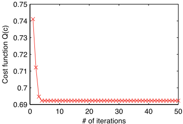
2 Typically, our proposed algorithm converges within five iterations on most datasets. Due to the page limit, we only report the convergence curve on the USPS dataset, as shown in Fig. 3.
includes 20 object classes, each of which contains 72 images; (3) SEGM [Frank and Asuncion, 2010] contains seven outdoor categories of images; (4) MFEAT [van Breukelen and Duin, 1998] contains 2,000 handwritten digital images from 0-9, which are extracted from the Dutch utility maps; (5) CAR [Bohanec and Rajkoviˇc, 1988] contains 1,728 textual records for evaluating cars based on price, safety, comfort and maintenance, which are categorized into four classes; (6) WAVE [Breiman et al., 1984] contains 5,000 textual instances sampled from three classes.
Compared Graphs. We compare four graph construction approaches including kNN graphs, neighborhood-fitted (Nfitted) graphs [Wang and Zhang, 2008], Sparsity Induced Similarity (SIS) graphs [Cheng et al., 2009], and our proposed M-fitted graphs. In kNN graphs, we use the Gaussian RBF kernel for weighting edges. For kNN and N-fitted graphs, we empirically set the number of nearest neighbors to k = 6. To build SIS graphs, for each instance we select its n 4c (c is the total number of classes) nearest neighbors to carry out ℓ1 minimization. For simplicity, we set m = n 4c and s = 6 to construct our M-fitted graphs.
Quantitative Results. To set up semi-supervised learning (SSL) trials, we uniformly sample instances at random from each dataset, ensuring that every class covers at least one instance. We denote by l the average number of labeled instances per class. On each dataset, we conduct 50 SSL trials. The SSL outputs are the classification error rates, averaged over 50 trials, achieved by different combinations of graph construction and SSL methods. We also report the average runtime 3 that every combination of graph construction and SSL takes.
3 All of our experiments are run on a workstation with INTEL
| Graph | COIL | SEGM | ||||||||
|---|---|---|---|---|---|---|---|---|---|---|
| l = 2 | USPS l = 5 Error/% | Time/s | l = 2 | l = 5 | Time/s | l = 2 | l = 5 Error/% | Time/s | ||
| Error/% | Error/% | Error/% | Error/% | |||||||
| kNN | 29.96 | 20.89 | 0.3580 | 9.65 | 4.91 | 1.5452 | 39.11 | 31.12 | 0.2785 | |
| N -Fitted | 31.29 | 22.28 | 7.8536 | 9.04 | 4.45 | 26.3985 | 38.58 | 30.97 | 8.5385 | |
| LGC SIS | 31.19 | 22.42 | 19.1036 | 8.18 | 5.89 | 281.5685 | 37.13 | 29.30 | 13.6618 | |
| M-Fitted | 29.80 | 21.20 | 5.0395 | 5.69 | 2.88 | 14.8532 | 36.33 | 28.81 | 4.3460 | |
| kNN | 24.53 | 17.96 | 0.7478 | 6.68 | 3.22 | 1.7054 | 33.11 | 27.36 | 0.7131 | |
| N -Fitted | 22.35 | 16.63 | 8.2643 | 4.96 | 4.19 | 26.1052 | 37.26 | 28.17 | 6.4655 | |
| LNP SIS | 20.71 | 16.51 | 19.4061 | 9.25 | 3.28 | 289.6741 | 31.62 | 26.10 | 9.3933 | |
| M-Fitted | 20.71 | 16.16 | 3.6660 | 4.68 | 2.91 | 20.0269 | 30.66 | 25.55 | 3.3524 | |
| kNN | 38.05 | 25.02 | 0.3333 | 8.18 | 3.97 | 1.5627 | 36.31 | 28.71 | 0.2579 | |
| N -Fitted | 38.65 | 22.77 | 8.4252 | 5.08 | 2.25 | 27.4328 | 38.55 | 28.66 | 7.1161 | |
| GFHF SIS | 45.50 | 28.72 | 13.3950 | 4.85 | 2.62 | 279.6863 | 37.53 | 28.48 | 7.3029 | |
| M-Fitted | 29.50 | 19.13 | 3.8513 | 3.77 | 1.97 | 11.6737 | 36.21 | 27.76 | 3.5579 | |
| kNN | 20.19 | 14.58 | 0.3355 | 6.13 | 3.10 | 1.5509 | 31.28 | 25.96 | 0.2628 | |
| GFHF + CMN | N -Fitted | 19.97 | 14.07 | 8.5836 | 3.61 | 1.90 | 26.2992 | 31.01 | 25.38 | 7.2184 |
| SIS | 22.15 | 14.35 | 15.8672 | 3.59 | 2.19 | 283.8451 | 31.41 | 25.33 | 6.9735 | |
| M-Fitted | 17.12 | 12.69 | 3.3283 | 2.89 | 1.61 | 12.2562 | 30.30 | 24.38 | 3.4812 | |
| SSL | MFEAT | CAR | WAVE | |||||||
|---|---|---|---|---|---|---|---|---|---|---|
| Method | Graph | l = 2 | l = 5 Error/% | Time/s | l = 20 | l = 50 | Time/s | l = 2 | l = 5 | Time/s |
| Error/% | Error/% | Error/% | Error % | Error/% | ||||||
| LGC | kNN | 25.50 | 16.70 | 0.4126 | 21.01 | 17.50 | 0.2589 | 34.12 | 30.67 | 1.6048 |
| N -Fitted | 27.53 | 18.20 | 11.2863 | 26.48 | 22.86 | 5.5986 | 32.59 | 28.59 | 34.0939 | |
| SIS | 25.26 | 16.98 | 40.2452 | 25.37 | 20.80 | 4.0573 | 33.27 | 29.69 | 32.8699 | |
| M-Fitted | 24.31 | 16.45 | 8.9988 | 18.93 | 13.77 | 2.9807 | 32.30 | 28.27 | 26.8215 | |
| LNP | kNN | 18.01 | 11.72 | 0.7811 | 32.96 | 28.02 | 0.4416 | 41.69 | 33.21 | 5.0517 |
| N -Fitted | 19.13 | 12.37 | 7.6312 | 36.69 | 29.77 | 4.9133 | 39.64 | 31.60 | 18.2306 | |
| SIS | 17.78 | 11.61 | 34.7508 | 30.07 | 26.32 | 4.5560 | 34.75 | 29.38 | 33.8275 | |
| M-Fitted | 16.99 | 11.53 | 5.9624 | 19.91 | 15.56 | 2.8392 | 32.62 | 29.21 | 13.5131 | |
| GFHF | kNN | 26.97 | 15.00 | 0.4077 | 28.12 | 23.02 | 0.2020 | 63.17 | 53.87 | 1.3322 |
| N -Fitted | 31.42 | 17.28 | 6.8102 | 28.81 | 26.27 | 5.0929 | 63.41 | 56.37 | 16.9751 | |
| SIS | 31.72 | 17.16 | 35.5183 | 25.24 | 25.08 | 2.5673 | 64.76 | 57.93 | 21.3485 | |
| M-Fitted | 26.77 | 13.88 | 6.0885 | 20.97 | 15.64 | 2.1755 | 59.32 | 49.48 | 11.1181 | |
| GFHF + CMN | kNN | 17.93 | 11.87 | 0.3997 | 46.12 | 33.84 | 0.2113 | 30.12 | 27.28 | 1.3483 |
| N -Fitted | 19.76 | 13.37 | 13.7010 | 52.53 | 41.37 | 4.7314 | 30.18 | 27.11 | 17.8843 | |
| SIS | 19.05 | 13.00 | 35.5608 | 40.83 | 27.76 | 2.6938 | 29.96 | 27.52 | 28.2256 | |
| M-Fitted | 17.25 | 11.16 | 6.2676 | 38.23 | 25.38 | 5.2851 | 29.67 | 26.69 | 12.2025 | |
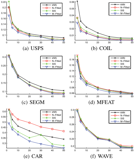
Tables 1, 2 and Figure 4 clearly show that our proposed M-fitted graphs lead to superior classification accuracy over the other graph construction approaches. In terms of the time cost, M-fitted graphs consistently run faster than the competing N-fitted and SIS graphs. Notice that M-fitted graphs always include the kNN search step, so they are slower than kNN graphs.
6 Conclusion and FutureWork
In this paper, we propose a sparse manifold fitting approach to embed the locally sparse manifold structure into neighborhood graph construction. In order to address the potential issues of ℓ1 relaxed sparse coding, our approach directly employs ℓ0 norm to induce sparsity, and designs a forwardbackward fitting algorithm to yield an explicitly sparse solution in an efficient manner. Through extensive experiments, we demonstrate the performance of the novel M-fitted graph generated by performing sparse manifold fitting for every input data point. M-fitted graphs not only run faster than stateof-art graphs, but also result in superior classification accuracy when collaborating with well-known graph-based semisupervised learning methods.
E5630 quad-core CPU and 48GB RAM. All methods mentioned in this paper are implemented in MATLAB.
In the future work, we would like to study scaling up the M-fitted graph proposed in this paper and enable it to work for massive datasets that are increasingly encountered in the current big data era. The prior work Anchor Graph [Liu et al., 2010] offers a good example, but it has not incorporated too much manifold information which would become more evident in large-scale data collections. If we developed a scalable graph construction approach such that the underlying manifold structure can be captured to a deeper extent, we could improve the performance of some popular graph-based web-scale applications such as ranking [Xu et al., 2011] and hashing [Liu et al., 2011b].
Acknowledgement:
This work is supported in part by Xiamen University 985 Project. Wei Liu is supported by the Josef Raviv Memorial Postdoctoral Fellowship.
@inproceedings{ijcai2013p280,
  title     = {Semi-Supervised Learning with Manifold Fitted Graphs},
  author    = {Zhang, Tongtao and Ji, Rongrong and Liu, Wei and Tao, Dacheng and Hua, Gang},
  booktitle = {Proceedings of the Twenty-Third International Joint Conference on
               Artificial Intelligence, {IJCAI-13}},
  publisher = {AAAI Press / International Joint Conferences on Artificial Intelligence},
  editor    = {Francesca Rossi},
  pages     = {1896--1901},
  year      = {2013},
  month     = {8},
  url       = {https://ijcai.org/proceedings/2013/280},
}
TY - CPAPER TI - Semi-Supervised Learning with Manifold Fitted Graphs AU - Zhang, Tongtao AU - Ji, Rongrong AU - Liu, Wei AU - Tao, Dacheng AU - Hua, Gang T2 - Proceedings of the Twenty-Third International Joint Conference on Artificial Intelligence, IJCAI-13 PB - AAAI Press / International Joint Conferences on Artificial Intelligence PY - 2013 SP - 1896 EP - 1901 UR - https://ijcai.org/proceedings/2013/280 ER -Copied
Machine-readable versions of this paper, for tools and AI agents:





