Disentangling Direct and Indirect Interactions in Polytomous Item Response Theory Models

1 Introduction

In this work, we study probabilistic models that are motivated by item response theory (IRT), see [Hambleton et al., 1991], and its applications in the social sciences. The goal of IRT is to indirectly measure latent personality traits such as economic behavior, intelligence, or well-being by using questionnaires. While classical IRT only considers the dichotomized outcomes right and wrong for each question, polytomous IRT, see [Ostini and Nering, 2006], allows more general discrete outcomes. Apart from right and wrong there can, for instance, be an additional no-choice option. Alternatively, all available options from multiple-choice questions can be taken into account. Hence, in general, IRT considers models with observed variables x from a discrete sample space X = ∏di=1 Xi, where the Xi = {0, . . . ,mi} are finite sets of choice options, and it additionally considers latent variables z from a continuous sample space Z = Rr . Here, the number r of latent variables is small in comparison to the number d of observed variables. Moreover, all variables are assumed to be random.

∗Contact Author

Since the assumption behind IRT is that the observed outcomes can be explained by the latent traits, any probabilistic IRT model must describe the interaction between the observed and the latent variables. The simplest (unnormalized) model that respects this requirement is given by

where the pairwise interaction between the observed and latent variables is modeled by the r × m matrix R. Here, m = ∑di=1 mi and we do not use the observed variables directly but encode them as concatenated indicator variables

where [n] = {1, . . . , n} for n ∈ N. In general, IRT studies strive for independent measurements of the latent traits, that is, the observed variables should be conditionally independent given the latent variables. However, as [Chen et al., 2018] have shown for classical dichotomous IRT, this assumption is often violated, resulting in potentially unjustified biases. It is safe to assume that the same also holds true for polytomous IRT. Hence, a more reasonable probabilistic model for IRT is a pairwise conditional Gaussian (CG) distribution, see [Lauritzen, 1996]. It is given by

where S ∈ Sym(m) are the symmetric direct interactions of the observed variables. From this joint model we can derive the marginal model for the observed discrete variables by integrating out the latent variables z as

where L = R⊤R has rank at most r. This shows that a small number of latent variables induces a pairwise low-rank interaction between the observed variables. We still assume that the conditional independence assumption of IRT is not violated much, that is, the observed variables are mostly independent conditioned on the latent variables. Here, any conditional dependence between two observed discrete variables is determined by a group of parameters within the matrix S of direct interactions. These groups are given as

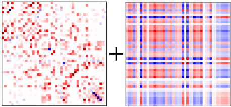
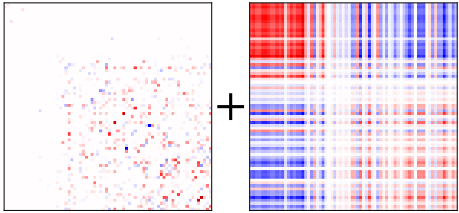
where the group Sij ∈ Rmi×mj contains the interaction parameters for the i-th and j-th observed variable. Hence, the absence of a direct pairwise interaction between two observed variables means that all parameters in the corresponding group are zero. Consequently, the assumption that most of the observed variables are conditionally independent implies group sparsity of S. Overall, the interaction between the observed variables in our marginal probabilistic IRT model is the sum of a group-sparse and a low-rank matrix, see Figure 1 for two examples.

For the proper analysis of IRT models, it is important to disentangle the group-sparse and low-rank interactions because only the low-rank interactions are induced by the latent variables, which are of primary interest here. Hence, the goal of this work is the design and analysis of a method for consistent estimation of the group-sparse and the low-rank part of the interaction matrix for the observed variables. Here, we use the classical maximum likelihood approach for estimating the interaction parameter matrix Θ = S + L of the discrete variables. To simplify our exposition, we minimize the convex negative log-likelihood function that can be derived from our model and reads as

where a(Θ) is the log-partition (normalization) function of the model and Σn = 1/n ∑nk=1 x(k) ⊗ x(k) is the empirical second-moment matrix that is computed as the average over outer products of n indicator-encoded observations x(k) ∈ {0, 1}m. Since by our assumptions the interaction matrix Θ is the sum of a group-sparse and a low-rank matrix, we promote this structure in the estimation process by adding group-sparsity and low-rank inducing regularization terms to the objective. First, it is well known that low rank can be induced on positive semidefinite L by trace-norm regularization tr(L). Second, group-sparse structure can be induced on S by ℓ1,2-norm regularization. Here, the ℓ1,2-norm is given by ‖S‖1,2 = ∑di,j=1 ‖Sij‖2, where, depending on the dimensions of Sij, the norm ‖Sij‖2 denotes the absolute value, the Euclidean vector norm, or the Frobenius norm. Hence, we study the following convex optimization problem

that uses regularization parameters λ, γ > 0. In Section 4, we will show that under some mild technical conditions, the solution to Problem (3) with appropriate regularization parameters can indeed consistently disentangle the group-sparse and the low-rank components of the interaction matrix.

2 Contributions and RelatedWork

A necessary condition for successful disentanglement of the group-sparse and low-rank components of the interaction matrix is that our model is identifiable. A parameterized class of probability distributions is identifiable if no distribution from the class has two different parameterizations. In our case this means that there should be no two group-sparse matrices S and S′ and two low-rank matrices L and L′ with (S,L) ̸= (S′ ,L′ ) such that S + L = Θ = S′ + L′ . In Sections 3 and 4, we work out conditions that ensure identifiability of our model.

The issue of identifiability received considerable attention in the context of mixture models, where the sample space Z of the latent variables is, in contrast to our model, a finite set. In this setting, the marginal distribution on the sample space X of the observed variables is a mixture of distributions p(x) = ∑z∈Z p(x, z) = ∑z∈Z p(z)p(x|z), where p(x|z) are the mixture components with corresponding weights p(z). A mixture model can be interpreted as a clustering of the observed samples into |Z| clusters, where the posterior p(z|x) is the probability that x belongs to cluster z ∈ Z. One must however be cautious with such an interpretation if there exists a different global model that yields the same marginal model. In this case, there is an identifiability problem since the joint models cannot be told apart from what can be observed, although they describe different clusterings. [Carreira-Perpinán and Renals, 2000], [Allman et al., 2009], and [Montúfar and Morton, 2017] provide conditions that ensure the identifiability of various mixture models.

Closer to our setting, [Candès et al., 2011] and [Chandrasekaran et al., 2011] provide conditions for the identifiability of matrix decompositions into sparse and low-rank components. [Tang and Nehorai, 2011] extend these conditions to column-sparse + low-rank matrix decompositions. In this work, we generalize the previous identifiability results to the group-sparse case that we motivated before.

Next, recall that a learning method is called consistent if it can recover the parameters of a probabilistic model in the limit of a growing number of data points that have been sampled from the model. Note that there cannot be a consistent learning method for non-identifiable models and thus the existence of a consistent learning method is a stronger property. [Ravikumar et al., 2011] and [Jalali et al., 2011], respectively, show that the parameters of Gaussian and discrete graphical models can be recovered consistently via convex optimization. In pioneering work, [Chandrasekaran et al., 2012] extend this approach to latent variable Gaussian graphical models, that is, to multivariate Gaussians with observed and latent variables. In previous work it was shown that consistent recovery is also possible for sparse + low-rank models with observed binary variables [Nussbaum and Giesen, 2019] and with mixed binary and conditional Gaussian observed variables [Nussbaum and Giesen, 2020]. Here, we extend their approach to group-sparse + low-rank interaction matrices. In Section 5, we corroborate our theoretical findings in experiments on synthetic data. Furthermore, we demonstrate the expediency of our model and model-selection approach on two polytomous IRT datasets from the social sciences.

3 Identifiability of the Model

In this section, we discuss the identifiability of the decomposition of the pairwise interaction parameter matrix from Model (1). For that, we consider group-sparse matrices that are contained in the group-sparse matrix variety of symmetric matrices with at most s non-zero groups given by

where gsupp(S) = {(i, j) ∈ [d] × [d] : Sij ̸≡ 0} defines the group support of S. Here, the groups Sij ∈ Rmi×mj are as in Equation (2). Moreover, we consider low-rank matrices from the low-rank matrix variety of symmetric matrices with rank at most r that is given by

Next, we provide a condition that ensures local identifiability of the product variety S(s) × L(r) for fixed s and r. We call (S, L) ∈ S(s)×L(r) locally identifiable if (S+∆, L-∆) /∈ S(s) × L(r) for all ∆ ̸= 0 from some small ball. Hence, we need to characterize nearby points in the varieties. First, if S ∈ S(s) with | gsupp(S)| = s, then S + ∆ ∈ S(s) for small ∆ if and only if ∆ is contained in the tangent space

to L(r), where L = UDU ⊤ is the (restricted) eigenvalue decomposition of L with U ∈ Rm×r and D ∈ Rr×r . This time, because the low-rank matrix variety is locally curved, having L - ∆ ∈ L(r) for small ∆ only implies that ∆ is a direction from some tangent space T (L′ ) to L(r) at a matrix L′ ∈ L(r) that is close to L. The following lemma shows that it is still sufficient to only consider T (L) for local identifiability.

Lemma 1. Let Q(S) ∩ T (L) = {0}, that is, we assume that the tangent spaces Q(S) and T (L) are transverse. Then, (S,L) is locally identifiable in S(s) × L(r), where s = | gsupp(S)| and r = rank(L).

To establish this result, one can prove that transversality of the tangent spaces extends to nearby tangent spaces. Now, restricting S(s)×L(r) to points (S, L) with Q(S) ∩T (L) = {0} leads to a class of locally identifiable models, though not globally identifiable. For example, using the first and m-th standard basis vectors of Rm, the pair consisting of S = e1e⊤1 and L = eme⊤m is locally identifiable in S(1)×L(1) since for d ≥ 2 it holds Q(S)∩T (L) = {0}. However, exchanging the roles of S and L yields a different parametrization (L, S) ∈ S(1) × L(1) of the same model.

The problem in the example is that both components are group sparse and low rank and thus can be confused. To avoid this, first the matrix S should have a small maximum degree gdegmax(S), that is, a small maximum number of non-zero groups per row/column. If this is the case, S cannot be mistaken as low rank. Second, the low-rank matrix L should have a row/column space U(L) ⊆ Rm that is not well-aligned with the standard-basis vectors ei of Rm. Formally, the incoherence coh(L) = maxi ‖PU(L)ei‖2 of L should be small because then L is spread-out and cannot be confused with a group-sparse matrix. The next lemma shows that bounding the product gdegmax(S) coh(L) implies tangent space transversality and thus identifiability by Lemma 1.

Lemma 2. Let (S,L) ∈ S(| gsupp(S)|) × L(rank(L)) and η = maxi∈[d] mi. Then, provided that it holds that gdegmax(S) coh(L) < 1/2η-3/2 , the tangent spaces Q(S) and T (L) are transverse, that is, Q(S) ∩ T (L) = {0}.

Observe that for (S,L) as in the previously discussed example it holds gdegmax(S) coh(L) = 1 such that the condition of Lemma 2 is not satisfied. In the next section, we will see that a slightly stronger upper bound on the product gdegmax(S) coh(L) even allows the consistent recovery of (S, L) by solving instances of Problem (3).

4 Consistency Analysis

For our consistency analysis we assume that n data points have been drawn from Model (1) with true interaction parameter matrix S⋆ + L⋆ , where S⋆ is group sparse and L⋆ is low rank. We show that the solution (Sn,Ln) to Problem (3) can recover the true parameters (S⋆ , L⋆ ) consistently, that is, asymptotically and with high probability. Specifically, we show two types of consistency. The first type is algebraic consistency. It holds if Sn has the same group support as S⋆ and if Ln has the same rank as L⋆ . The second type is parametric consistency, which holds if the errors Sn - S⋆ and Ln -L⋆ are small. Following [Chandrasekaran et al., 2012], a good measure for the size of the errors is the dual norm of the regularizing norm γ‖S‖1,2 + ‖L‖∗ from the objective function. We call this dual norm the γ-norm. It is given by

for (M,N) ∈ Sym(m) × Sym(m), where ‖M‖∞,2 = maxi,j ‖Mij‖2, and ‖N‖ is the spectral norm of N.

Consistent recovery is not always possible. A first challenge is controlling the sampling error, which is given by ∇ℓ(S⋆ + L⋆ ) = ∇a(S⋆ + L⋆ ) - Σn = E[Σ] - Σn , where the expectation is w.r.t. the true model. If the sampling error is small, then the likelihood term in Problem (3) ensures that the compound matrix Sn + Ln is close to the true compound matrix S⋆ +L⋆ . However, reliable recovery of the compound matrix is only possible if λ is not too large. Indeed, the regularization terms should only encourage small adjustments to the algebraic structure of the components. Hence, later we assume an upper bound on λ.

A second challenge is telling the group-sparse and lowrank components apart. This can be addressed by restricting the analysis to identifiable models as outlined in Section 3. For a better understanding, let us consider the intuitive variety-constrained version

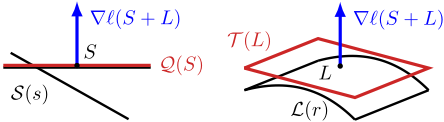
of Problem (3). This non-convex problem is of a hypothetical nature because the true group-sparse and low-rank matrix varieties with s = | gsupp(S⋆ )| and r = rank(L⋆ ) are unknown when solving the problem. Nevertheless, Problem (3) can be seen as a convex relaxation of the variety-constrained problem. Therefore intuitively, the solution of the varietyconstrained problem should be (locally) unique in order to successfully recover the true parameters. The main reason for local non-uniqueness can be a decomposition S + L that is not locally identifiable. This can be excluded by Lemma 1 provided that Q(S) ∩ T (L) = {0}. However, we must also ensure that no nearby solutions with different compound matrices exists. To fully characterize local uniqueness, we use the optimality conditions of the variety-constrained problem, see Figure 2. They state that (S, L) can only be a (local) solution if the gradient of the negative log-likelihood at S +L is normal to the respective varieties, that is, if it holds that

Here, the gradient is the same with respect to S and L. To guarantee local uniqueness, the optimality condition should be violated at any slightly perturbed solution, that is, the gradient at such a perturbed solution should be non-normal to at least one of the varieties.

In what follows, we focus on perturbations in tangential directions since the normal spaces to the varieties hardly change for such perturbations. Hence, for a tangentially perturbed solution, the optimality conditions are surely violated if the gradient at the perturbed solution has components in the tangent spaces that are large compared to the components in the normal spaces. Therefore, we need to control the change of the gradient under small (tangential) perturbations ∆. It is sufficient to do this only for perturbations from the true solution (S⋆ ,L⋆ ) since our assumptions will carry over to any nearby local solution (S,L). Now, given a small sampling error ∇ℓ(S⋆ +L⋆ ), the change of the gradient is locally governed by the Hessian H⋆ = ∇2 ℓ(S⋆ + L⋆ ). This follows from the first-order approximation

Consequently, the tangential components of the gradient at the perturbed solution are large if the minimum gains of the Hessian H⋆ in tangential directions are large. At the same time, the normal components of the gradient are not too large if the orthogonal effects of the Hessian H⋆ in normal directions are not too large compared to the tangential effects. We formalize this in our main assumption.

Assumption 1. We assume that there exist α > 0, ν ∈ (0, 1/2], and an interval [γmin, γmax] such that the following holds for any γ ∈ [γmin, γmax], any (low-rank) tangent space T (L′ ) that is sufficiently close to T (L⋆ ), and any (M, N) ∈ J = Q(S⋆ ) ×T (L′ ): First, the minimum gain on J of H⋆ is bounded from below in the sense that

where D : Sym(m) → Sym(m) × Sym(m), M ↦→ (M, M) is the duplication operator. Second, the orthogonal effect on J ⊥ of H⋆ is bounded from above in the sense that

A few comments are in order to understand this assumption. First, note that Assumption 1 is a generalization of the irrepresentability assumption as for example used by [Zhao and Yu, 2006, Wainwright, 2009, Ravikumar et al., 2011]. Second, Assumption 1 concerns tangent spaces that are close to T (L⋆ ) to account for the local curvature of the low-rank matrix variety. Third, the assumption on the minimum gain implies transversality, that is, Q(S⋆ ) ∩ T (L′ ) = {0}. In conjunction with Lemma 1, this entails local identifiability. Fourth and finally, it can be shown that the existence of the interval [γmin, γmax] is implied by the upper bound gdegmax(S⋆ ) coh(L⋆ ) ≤ c/12η-3/2 (αν)2 (2 - ν)-2 that uses the constants α and ν from the assumption as well as another constant c that is independent of n and d. Recall that in Section 3 we have seen that small gdegmax(S⋆ ) and coh(L⋆ ) help to avoid confusion of S⋆ and L⋆ . Hence, assuming an upper bound on gdegmax(S⋆ ) coh(L⋆ ) is reasonable.

Next, we formulate our consistency result, assuming a small sampling error first. We control the sampling error by a probabilistic analysis afterwards. Moreover, for better readability, we leave out constants that are independent of n, d, the group sparsity of S⋆ , and the coherence of L⋆ . We denote inequalities that hold up to such constants by ≲ and ≳.

Theorem 1. Let S⋆ ,L⋆ ∈ Sym(m) with L⋆ ⪰ 0 such that Assumption 1 is satisfied. Suppose that we observed samples x(1) , . . . , x(n) ∈ X drawn from Model (1) with interaction matrix S⋆ + L⋆ . Assume that λ≲ coh(L⋆ ), that γ ∈ [γmin, γmax], and that the sampling error is bounded as

Also assume that the minimum magnitude of the nonzero groups of S⋆ is bounded from below as smin = min(i,j)∈gsupp(S⋆ ) ‖Sij‖2 ≳λ| gsupp(S⋆ )|-1d and that the minimum non-zero singular value of L⋆ is bounded from below as σmin ≳λcoh(L⋆ )-1 . Then, it follows that the solution (Sn, Ln) to Problem (3) with regularization parameters λ and γ is unique and

(a) parametrically consistent in the sense that it satisfies ‖(Sn - S⋆ , Ln - L⋆ )‖γ ≲ λ and

(b) algebraically consistent, that is, Sn and S⋆ have the same group support, and Ln and L⋆ have the same rank.

We make a few additional comments concerning the assumptions of Theorem 1. First, recall that an upper bound on λ is needed for reliable recovery of the compound matrix S⋆ + L⋆ . We also assume lower bounds on smin and σmin in terms of λ to avoid that the shrinkage effects due to the regularization cause algebraic features of the decomposition to disappear. Next, it is natural to require the sampling error to be bounded by λ since intuitively, for large λ and thus strong regularization, we can allow for a larger sampling error. However, while the probability that the sampling-error bound holds for an actual sample will also be larger for large λ, the error bound in Theorem 1(a) gets weaker.

Similarly as in [Chandrasekaran et al., 2012] and [Nussbaum and Giesen, 2020], Theorem 1 can be proven using the primal-dual witness technique: It proceeds by first restricting Problem (3) to a (non-convex) correct model set M that is chosen in a way such that any solution (SM,LM) to the restricted problem is algebraically and parametrically consistent. The non-convexity is due to a rank constraint, which is subsequently replaced by a linear tangent-space constraint to the low-rank matrix variety at a fixed solution (SM, LM). Then, it is shown that the solution to the linearized problem is unique and coincides with (SM,LM). Finally, it is shown that the original Problem (3) is also solved by the same consistent solution (SM, LM).

Next, we show that the bound on the sampling error that is required by Theorem 1 holds with high probability for a specific choice of λ.

Corollary 1. Under the assumptions of Theorem 1 let

for some κ ≥ 1 and let n≳κη2 coh(L⋆ )-4d logm. Then, it follows that ‖D(E[Σ] -Σn )‖γ ≲λn,d with probability at least 1 -m-κ . Hence, the conclusions of Theorem 1 applied with λ = λn,d hold with the same probability.

Corollary 1 can be proven using concentration results for bounded random vectors [Vershynin, 2010]. The dependence on coh(L⋆ ) can be improved in both Theorem 1 and Corollary 1 in a rather technical and non-intuitive way. However, here we choose to remain clear and self-contained. We investigate the influence of coh(L⋆ ) and gdegmax(S⋆ ) in our experiments in the next section.

The specific choice λ = λn,d in Corollary 1 allows the discussion of some high-dimensional limits. For that we consider problems that vary in the number of data points n, in the number of observed variables d, and in the group sparsity and the incoherence of the components. Apart from that, we only consider problems that satisfy the assumptions from Theorem 1 for the same constants, particularly the same α and ν. In this setting, first observe that for fixed d the error bound ‖(Sn - S⋆ , Ln - L⋆ )‖γ ≲ λn,d from Corollary 1 asymptotically approaches zero as n →∞. Second, for larger d, more samples are required to obtain the same error bound. Furthermore, we expect that larger gdegmax(S⋆ ) and larger coh(L⋆ ) make consistent recovery more difficult since then it is more likely that the upper bound on gdegmax(S⋆ ) coh(L⋆ ) is not satisfied. We also investigate this in our experiments.

5 Experiments

We solve Problem (3) using the Alternating Direction Method of Multipliers (ADMM) with a proximal gradient step that we adapted to our needs from [Ma et al., 2013]. For computational efficiency, we replace the likelihood by the pseudolikelihood in our experiments. It is known to behave similarly [Mozeika et al., 2014].

5.1 Synthetic Data

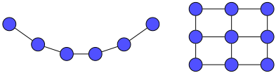
Here, to verify experimentally that consistent recovery is possible, we generate synthetic data from discrete fused latent and graphical models using Gibbs sampling, see [Casella and George, 1992]. For the experiments, we use discrete variables that take three values, that is, Xi = {0, 1, 2} for all variables. We consider four models with d = 36 variables, where the direct interactions S⋆ adhere to either chain or grid graphical model structures (compare Figure 3), and the number of latent variables is either one or two.

Our goal is to test the influence of the maximum group degree gdegmax(S⋆ ) of S⋆ and the incoherence coh(L⋆ ) of L⋆ on recovery rates. Here, the maximum group degree is two for the chain and four for the grid model. Moreover, we set the probability of an interaction between any latent and any observed variable to be non-zero to 95%. This ensures that the low-rank effect of the latent variables is spread-out and thus that L⋆ is incoherent. However, L⋆ will be less incoherent for a growing number of latent variables.

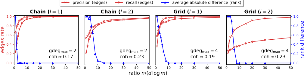
For each model, we sample all of its parameters randomly. More specifically, we sample the latent-observed interaction parameters uniformly from [-0.5, -0.2] ∪ [0.2, 0.5] and the parameters for the non-zero groups of S⋆ from [-1.5, -0.5] ∪ [0.5, 1.5]. Then, for each model we test the asymptotic behavior by generating 20 datasets with kd log m samples (rounded to the nearest integer) for selected ratios k ∈ [1, 50]. Our choice of regularization parameters is guided by Corollary 1 and fixed for all models (λ = 1/50 √d logm/n, γ = 10). Finally, for each model and ratio k, we record the average percentage of correctly identified non-zero groups, that is, edges in the conditional independence graph. For that, we employ the criteria of recall and precision, where recall = TP/(TP+FN) and precision = TP/(TP+FP). Here, TP is the number of correctly identified edges (true positives), FN is the number of undetected edges (false negatives), and FP is the number of edges that were mistakenly detected as edges (false positives). Likewise, we record the absolute rank difference | rank(Ln) - rank(L⋆ )|, averaged over the 20 trials.

The results are shown in Figure 4. Recovery of edges and rank requires relatively few samples for the one-latentvariable chain and grid models. Slightly more samples are required to recover the rank of the grid model. This is due to the larger maximum group degree of the grid models compared to the chain models. Next, for the two-latent-variable chain model considerably more samples are necessary for successful recovery-because the underlying low-rank matrix is less incoherent. Our observations back the intuition that for more incoherent L⋆ and smaller maximum group degree of S⋆ , the group-sparse and low-rank components can be confused less easily. This is supported even more by the recovery results for the two-latent-variable grid model, where the fact that both the maximum group degree and the coherence are larger is reflected in significantly worse recovery results. Nevertheless, overall the results show that consistent recovery is possible.

5.2 Real-World Data

We also demonstrate the effectiveness of our fused latent and graphical models on two real-world datasets. The first dataset is from a non-forced choice vocabulary IQ test (VIQT), where participants can indicate if they do not know an answer, otherwise answers are either correct or wrong. The dataset was obtained from the [Open-Source Psychometrics Project, 2019] and contains d = 45 variables and n = 12 173 samples. The second dataset contains the answers of n = 165 test takers to the d = 72 questions of the Cambridge face memory test (CFMT) [Duchaine and Nakayama, 2006,Itz et al., 2017]. In this dataset, answers with response times below the human reaction time or above some threshold (based on the interquartile range) were assigned to a third category of outliers, otherwise answers are either correct or wrong, again. Hence, for both datasets, the observed variables are discrete with three possible outcomes.

Figure 1 shows estimated fused latent and graphical models for both datasets. The learned models exhibit direct interactions, that is, the answers are not independent given the estimated latent variables. This is in contrast to the common conditional independence assumption in item response theory. Nevertheless, for both models, most observed interactions are explained by a latent variable. Notably, the low-rank matrix learned for the CFMT data has a block of positively correlated items in the top left corner. These items correspond to the first CFMT block, which consists of 18 simple questions that most participants get right, hence the correlation.

6 Conclusion

In this paper, we studied discrete fused latent and graphical models. We investigated when the group-sparse + low-rank decomposition of the interaction parameter matrix is identifiable. We showed that using convex optimization such decompositions can be estimated consistently in the highdimensional setting. We verified experimentally that consistent recovery becomes easier if there are not too many non-zero groups per row/column of the matrix of direct interactions and if the low-rank matrix is spread-out. The fused latent and graphical models that we estimated from real-world data demonstrate that observed data from polytomous IRT studies can be conditionally dependent given the latent variables-in contrast to the common assumption. This shows that modeling direct interactions in polytomous IRT is warranted and reasonable.