
Logics of Allies and Enemies: A Formal Approach to the Dynamics of Social Balance Theory
Proceedings of the Twenty-Ninth International Joint Conference on Artificial Intelligence. Main track. Pages 210-216.
https://doi.org/10.24963/ijcai.2020/30
Keywords
- Agent-based and Multi-agent Systems: Agent Societies
- Multidisciplinary Topics and Applications: Social Sciences
Abstract
We combine social balance theory with temporal logic to obtain a Logic of Allies and Enemies (LAE), which formally describes the likely changes to a social network due to social pressure. We demonstrate how the rich language of LAE can be used to describe various interesting concepts, and show that both model checking and validity checking are PSPACE-complete.
- [Abell and Ludwig, 2009] Peter Abell and Mark Ludwig. Structural balance: A dynamic perspective. The Journal of Mathematical Sociology, 33(2):129-155, 2009.
- [Antal et al., 2006] Tibor Antal, Paul L. Krapivsky, and Sid- ney Redner. Social balance on networks: The dynamics of friendship and enmity. Physica D: Nonlinear Phenomena, 224(1-2):130-136, December 2006.
- [Baltag et al., 2019] Alexandru Baltag, Zoé Christoff, Ras- mus K. Rendsvig, and Sonja Smets. Dynamic epistemic logics of diffusion and prediction in social networks. Stu- dia Logica, 107(3):489-531, 2019.
- [Cartwright and Harary, 1956] Dorwin Cartwright and Frank Harary. Structure balance: A generalization of Heider's theory. Psychological Review, 63(5):277-293, September 1956.
- [Christoff and Hansen, 2015] Zoé Christoff and Jens Ulrik Hansen. A logic for diffusion in social networks. Jour- nal of Applied Logic, 13(1):48 -77, 2015.
- [Clarke and Emerson, 1981] Edmund M. Clarke and E. Allen Emerson. Design and synthesis of synchroniza- tion skeletons using branching time temporal logic. In Dexter Kozen, editor, Logics of Programs, pages 52-71, Berlin, Heidelberg, 1981. Springer Berlin Heidelberg.
- [Doreian et al., 1996] Patrick Doreian, Roman Kapuscinski, David Krackhardt, and Janusz Szczypula. A brief history of balance through time. The Journal of Mathematical So- ciology, 21(1-2):113-131, 1996.
- [Emerson and Clarke, 1982] E.Allen Emerson and Ed- mund M. Clarke. Using branching time temporal logic to synthesize synchronization skeletons. Science of Computer Programming, 2(3):241-266, 1982.
- [Harary et al., 1965] Frank Harary, Robert Z. Norman, and Dorwin Cartwright. Structural Models: An Introduction to the Theory of Directed Graphs. John Wiley & Sons Inc, New York, September 1965.
- [Harary, 1953] Frank Harary. On the notion of balance of a signed graph. Michigan Mathematical Journal, 2(2):143- 146, 1953.
- [Heider, 1944] Fritz Heider. Social perception and phenome- nal causality. Psychological Review, 51(6):358-374, 1944.
- [Heider, 1946] Fritz Heider. Attitudes and cognitive organi- zation. Journal of Psychology, 21(1):107-112, 1946.
- [Heider, 1958] Fritz Heider. The Psychology of Interper- sonal Relations. John Wiley & Sons, 1958.
- [Hummon and Doreian, 2003] Norman P Hummon and Patrick Doreian. Some dynamics of social balance processes: bringing Heider back into balance theory. Social Networks, 25(1):17-49, 2003.
- [Kulakowski, 2007] Krzysztof Kulakowski. Some recent at- tempts to simulate the Heider balance problem. Comput- ing in Science and Engineering, 9:80-85, 06 2007.
- [Newcomb, 1961] Theodore M. Newcomb. Acquaintance Process. Holt, Rinehart & Winston, New York, Decem- ber 1961.
- [Pedersen et al., 2019] M.Y. Pedersen, Sonja Smets, and Thomas Ågotnes. Analyzing echo chambers: A logic of strong and weak ties. In Proceedings of LORI 2019, pages 183-198, 2019.
- [Radicchi et al., 2007] Filippo Radicchi, Daniele Vilone, Sooeyon Yoon, and Hildegard Meyer-Ortmanns. Social balance as a satisfiability problem of computer science. Physical Review E, 75:026106, Feb 2007.
- [Stockmeyer and Meyer, 1973] L. J. Stockmeyer and A. R. Meyer. Word problems requiring exponential time (pre- liminary report). In Proceedings of the Fifth Annual ACM Symposium on Theory of Computing, pages 1-9, 1973.
- [van der Hoek et al., 2019] Wiebe van der Hoek, Louwe B. Kuijer, and Yì N. Wáng. Who should be my friends? so- cial balance from the perspective of game theory. In Pro- ceedings of LORI 2019, pages 370-384, 2019.
- [Wang and Thorngate, 2003] Zhigang Wang and Warren Thorngate. Sentiment and social mitosis: Implications of Heider's balance theory. Journal of Artificial Societies and Social Simulation, 6(3):12-23, June 2003.
- [Xiong and Ågotnes, 2019] Zuojun Xiong and Thomas Ågotnes. On the logic of balance in social networks. Journal of Logic, Language and Information, 29:53-75, 2019.
- [Zheng et al., 2015] Xiaolong Zheng, Daniel Zeng, and Fei- Yue Wang. Social balance in signed networks. Information Systems Frontiers, 17(5):1077-1095, January 2015.
References were extracted automatically from the PDF and may contain errors.
Full text extracted automatically from the PDF; figures, tables and equations may differ. The PDF is the version of record.
1 Introduction
Social balance theory was initiated with Heider's work on social psychology [1944; 1946; 1958], and later reinvented by Harary et al. using graph theory in [Harary, 1953; Cartwright and Harary, 1956; Harary et al., 1965], an approach in which signed graphs represent social networks of agents, with positive signs for allies or friends and negative signs for enemies or antagonists. This has become a basic framework for studying positive and negative ties, and has since then become an active area in the field of social network analysis.
A social network is balanced if it meets certain structural conditions on its positive or negative ties between agents. For example, a triad of three agents that are all enemies of one another is considered unbalanced, since two of them have an incentive to make an alliance against the third. Over time, the ties in a social network tend to change in a way that makes the network more balanced. Empirical and theoretical studies of social balance can be found in [Newcomb, 1961; Doreian et al., 1996; Hummon and Doreian, 2003; Wang and Thorngate, 2003; Antal et al., 2006; Radicchi et al., 2007; Kulakowski, 2007; Abell and Ludwig, 2009; Zheng et al., 2015].
Here we study the process under which networks become more balanced from a different perspective, namely that of temporal logic. Specifically, we introduce the Logic of Allies and enemies (LAE), a variant of Computation Tree Logic (CTL) [Clarke and Emerson, 1981; Emerson and Clarke, 1982] that describes the behaviour of social networks under the assumption that they move towards balance "greedily", i.e., that change in relations between agents happens only if it makes the network more balanced.
LAE allows us to describe properties of networks such as, for example, "it is guaranteed that a and b eventually become friends", "if a and c ever become friends, then they will remain friends forever, and a and b will forever be enemies" and "a and b will remain enemies until there are at least two agents x and y that are mutual friends of a and b". Our main results are that (1) it is possible for a social network to get stuck in a local maximum of balance, (2) the so-called balance theorem or structure theorem, which states that a network is balanced iff it is clique divisble, holds for LAE, and (3) model checking and validity checking for LAE are PSPACE-complete.
The structure of the paper is as follows. We introduce the basic ideas of network balance in the next section. In Section 3 we introduce the syntax and semantics of LAE, together with a number of validities; we also show that the movement towards balance may terminate in a state that is not fully balanced but instead only stable. We study the computation complexity in Section 4 and conclude in Section 5.
2 Network Balance
A social network consists of a set of agents with pairwise ties that are positive ("friends", "allies", +), negative ("foes", "enemies", -) or neutral ("neither friends nor foes", 0).
While every relation is between exactly two agents, the different relations do influence one another. For example, one of these influences is famously expressed by the saying that "the enemy of my enemy is my friend", so if there is enmity between a and b and between b and c, then there should be a friendship between a and c. There are multiple equivalent ways to describe these influences; our description is based on balanced and unbalanced triads. 1 Modulo symmetry there are 10 different triads, which are drawn in Figure 1.
We call a triad balanced if its edges reinforce each other. For example, in the triad --+ of Figure 1(b), the + edge between a and c is reinforced because b is a mutual enemy, the
- edge between a and b is reinforced because a is the friend of b's enemy c and the - edge between b and c is reinforced because c is the friend of b's enemy a. The two balanced triads are the aforementioned --+ and the triad +++.
1 The term "triad" is commonly used in the field of balance theory for a group of three agents and their relations. The study of triads was rooted in Heider [1944; 1946]. Influences from a bigger cycle are typically considered to be of less strength, and modeled in this paper by indirect cross-triad interaction over time.
Pressure-free
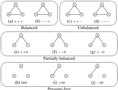
We call a triad unbalanced if all its edges weaken one another. For example, in the --- triad of Figure 1(d) each pair of agents has reason to become friendly to one another against a common foe. The other unbalanced triad is ++-.
There are also three triads where two of the edges are neither reinforced nor weakened, while a third edge experiences some pressure one way or the other. We call these triads partially balanced. E.g., in the triad --0 of Figure 1(f), there is no reason for the enmity between a and b or between b and c to end. But there is a reason for the neutrality between a and c to turn into a friendship, since they have b as a common foe.
Finally, the remaining three triads are pressure-free. In these triads 000, +00, -00, there is no pressure on any of the edges to change.
The different types of triads and the pressures they experience are summarized as follows:
| Degree of balance | Shape | Has a reason to change to . . . |
|---|---|---|
| Balanced | +++ +-- | N/A N/A |
| Unbalanced | ++- --- | -+-, +-- or +++ +--, -+- or --+ |
| Pressure-free | 000 +00 -00 | N/A N/A N/A |
| Partially balanced | ++0 --0 +-0 | +++ --+ +-- |
2.1 Scope
Balance theory models the influence that different relations in a social network have on one another. But the relations may be influenced by other factors as well. For example, "John may be the enemy of my enemy, but he punched me in the face yesterday so he is definitely not my friend" is a reasonable attitude, but does not follow from any of the relations in the network. Since such influences originate from factors that are not represented in the network, we refer to them as outside influence.
✔
✕
✔
Predicting outside influence would require an accurate model of all human behavior, which seems rather unfeasible and is outside the scope of balance theory, and of this paper. We therefore do not model outside influence. The network dynamics that we represent here are therefore best seen as the likely changes in the social network provided that there are no influences from outside the network.
3 The Logic of Allies and Enemies
✕
✔
In this section we first introduce formal definitions of 3signed social networks, stability scores and time evolution, based on the understanding and convention from the previous section. Then we introduce the syntax and semantics of the Logic of Allies and Enemies (LAE).
✕
We assume that every social network is finite, so let a finite set AG be given. Furthermore, because there is no reason for relations to change unless there are at least three agents, we assume that |AG| ≥ 3.
3.1 3-Signed Social Networks
We define a social network to be a 3-signed undirected graph, with its vertices representing agents and edges representing ties between agents. The formal definition is given below.
Definition 1 (social networks). A social network (network for short) is a function N : {{a, b} ⊆ AG : a ̸= b} → {+, -, 0} that assigns to each pair of different agents a positive (+), a negative (-), or a neutral (0) edge.
Note that the domain of N consists of unordered pairs of two different agents. We therefore have N({a, b}) = N({b, a}), by definition. We write N(a, b) for N({a, b}). We say that a network is complete if it does not contain neutral edges, and that two agents are in the same connected component if they are connected by a path of non-neutral edges.
We first introduce the notion of balance coming from the literature. That is, a network is balanced if all of its triads are balanced.
Definition 2 ((semi-)balance). A network N is balanced if for every distinct a, b, c ∈ AG, the triad abc is balanced in N. A network N is semi-balanced if for every distinct a, b, c ∈ AG, the triad abc is balanced or pressure-free in N.
The relation between the two concepts is characterized by the following proposition.
Proposition 3. A network is semi-balanced if and only if all of its connected components are balanced.
A network is semi-balanced if and only if no agent has any reason to change any of its relations. However, it is possible for two agents a and b to have both some reasons to become or remain friends, and some reasons to become or remain enemies. So the mere fact that an agent has a prima facie reason to change its relation does not mean that the agent has an overall reason to change its relation, since the reason for change may be outweighed by more reasons for the relation to remain the same. As a result, it is possible for a network not to be balanced, while still not containing any overall reason for any relation to change. We therefore introduce the notion of stability: a network is unstable if there is at least one pair of agents that have more reasons to change their relationship than they have reasons for it to remain the same.
The stability of an edge is determined by its attraction and repulsion. The attraction between two agents is the number of reasons for them to become or remain friends, and the repulsion the number of reasons to remain or become enemies.
This means that the attraction between a and b is the number of mutual friends/foes, while the repulsion is the number of agents to which a and b have different non-neutral ties.
Definition 4 (stability of edges). Let N be a social network, and let a, b ∈ AG. The attraction, repulsion and stability score of (a, b), denoted attr(a, b), rep(a, b) and score(a, b), respectively, is given by
An edge ab is stable if score(a, b)≥0, and unstable otherwise. An unstable edge is improving if its attraction is greater than repulsion, and deteriorating if attraction less than repulsion.
Put in a different way, a positive edge is unstable if it is deteriorating, a negative edge is unstable if improving, and a neutral edge is unstable if either deteriorating or improving.
Definition 5 (stability of networks). A network is stable if every edge is stable, and unstable otherwise. The stability score of a network N is the sum of the stability scores of its edges. We write score(N) for the stability score of N.
It is easy to see that every semi-balanced network is stable: if no edge has any reason to change, then, in particular, no edge has more reasons to change than to remain the same. The converse does not hold, however.
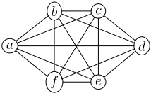
For example, the network shown in Figure 2 is stable but not balanced. For every edge in this network the agents have a reason to change their relation, but also a countervailing reason to keep their current relation. E.g., a and b might wish to become friends due to their common friendship with c and e, but they also wish to remain enemies due to the fact that d and f are enemies of b but friends of a.
Proposition 6. The set of semi-balanced networks is a proper subset of the set of stable networks.
If a network is unstable, one or more relations have more reasons to change than to remain the same. In such a situation, we expect one of these relations to change accordingly.
If a network is stable, then no relation has an overall reason to change, so the network is expected to remain the same. It follows that while networks trend towards balance, they may get stuck in a stable but not semi-balanced state.
Definition 7 (successors). We say a network N2 is a successor of a network N1 if: (i) N1 is stable and N1 = N2, or (ii) N1 and N2 differ in exactly one edge ab, and for that edge it is either the case that ab is improving in N1 and N2(a, b) = +, or that ab is deteriorating in N1 and N2(a, b) = -. We write N1 ❀N2 if N2 is a successor of N1.
Proposition 8. Let N1 and N2 be two networks such that N1 ❀N2. Then,
- If N1 is stable, then score(N1) = score(N2);
- If a neutral edge of N1 becomes positive or negative in N2, then score(N1) can be greater than, equal to or smaller than score(N2) (all cases can indeed occur);
- If a positive (resp. negative) edge of N1 becomes negative (resp. positive) in N2, then score(N1)<score(N2).
Definition 9. The time evolution T(N) of a network N is the smallest graph (S,⇒) such that: (i) N ∈ S, and (ii) if N1 ∈ S and N1 ❀ N2, then N2 ∈ S and N1 ⇒ N2.
Proposition 10. The time evolution of a network is a tree-like structure, i.e., there are no cycles except self-loops of leaves.
Proof. By Prop. 8 the only cycles are self-loops, i.e., of the form N1 ❀ N1, where N1 is stable. This is because whenever N1 ❀ N2 and N1 ̸= N2, either N2 contains strictly fewer neutral edges than N1, or N1 and N2 have the same number of neutral edges and score(N1) < score(N2).
We abuse notation by saying that T(N) has a depth, namely the length of the longest cycle-free path.
Proposition 11. The depth of any time evolution is bounded from above by 2 · |AG|5 .
Proof. Each reason for an edge to improve or deteriorate can be identified by a triad abc, where ab and bc influence ac. There are less than |AG|3 such triples, so the stability score must be between -|AG|3 and |AG|3 . Furthermore, there are at most |AG|2 edges with value 0. Since every non-reflexive transition requires either one edge to become non-neutral or the stability score to increase, the maximum cycle-free path length is at most 2 · |AG|3 · |AG|2 = 2 · |AG|5 .
3.2 Syntax and Semantics
We wish to reason about social networks and their evolution with a logical language. As T(N) strongly resembles the branching time models of CTL, we base the temporal connectives of our language on those of CTL. In addition to these temporal connectives we use a number of atoms that describe the ties. Because it is important for the network dynamics how many mutual friends/foes two agents have, we also use a quantifier ∃≥nx that allows us to describe how many agents satisfy a certain property.
Definition 12 (languages). The language L of LAE is given by the following grammar:
where a, x ∈ AG and n ∈ N. We use the Boolean operators ∧, ∨, ⊤ and ⊥ as well as the CTL operators EX, AF, EF, AG
and EG as abbreviations as usual. Pab reads as "the relation between a and b is positive, and Nab as "the relation between a and b is negative". Oab abbreviates (¬Pab ∧ ¬Nab), and reads as "the relation between a and b is neutral". With regard to the quantifier, ∃≥nxϕ reads as "there are at least n agents x such that ϕ(x) is true." We will make use of the following abbreviations:
∃xϕ =df ∃≥1xϕ ∀xϕ =df ¬∃x¬ϕ ∃!nxϕ =df (∃≥nxϕ∧¬∃≥n+1xϕ)For simplicity we treat Pab and Pba as the same formula, and similarly for the operators N and O.
Formally, the meaning of the formulas is determined by the satisfaction relation |=, which is defined as follows.
Definition 13 (satisfaction). Whether a network N satisfies (notation N |=) a formula is determined inductively by the following (where ϕ and ψ are formulas, and a, b, x ∈ AG):
N |= Pab iff N(a, b) = + N |= Nab iff N(a, b) = - N |= ¬ϕ iff not N |= ϕ N |= (ϕ→ψ) iff N |= ϕ implies N |= ψ N |= AXϕ iff ∀N ′ : N ❀N ′ implies N ′ |= ϕ N |= A(ϕUψ) iff ∀N1, · · · , if N0 ❀N1 ❀ · · · with N =N0, then ∃i : Ni |= ψ and ∀j < i,Nj |= ϕ N |= E(ϕUψ) iff ∃N1, · · · such that N0 ❀N1 ❀ · · · N =N0, and ∃i : Ni |= ψ and ∀j < i,Nj |= ϕ N |= ∃≥nxϕ iff there are distinct a1, . . . , an ∈ AG such that N |= ϕ[ a1 x ] ∧ · · · ∧ ϕ[ an x ],where ϕ[ ai x ] (for all i = 1, . . . , n) is the formula achieved by substituting all occurrences of x in ϕ to ai.
A formula is satisfiable if there is a network that satisfies it, and valid if all networks satisfy it.
Our logic is strong enough to express stability of edges and networks and balance of triads and networks:
stable(a, b) =df (Pab∧AXPab) ∨ (Nab∧AXNab) ∨(Oab∧AXOab) stable =df ∀xy stable(x, y) noneutral(a, b, c) =df ¬(Oab ∨ Obc ∨ Oac) balanced(a, b, c) =df (Pab∧Pbc∧Pca)∨(Pab∧Nbc∧Nca) ∨(Nab∧P bc∧Nca)∨(Nab∧Nbc∧P ca) balanced =df ∀xyz(noneutral(x, y, z) → balanced(x, y, z)) ∧∀x¬∃≥2yOxywhere stable(a, b) intuitively says that the edge ab is stable, stable says that the current network is stable (N |= stable iff N is stable), noneutral(a, b, c) says that abc contains no neutral edges, balanced(a, b, c) says that abc is a balanced triad (positive 3-cycle), and balanced says that the current network is balanced (N |= balanced iff N is balanced). Semi-balance can also be expressed in LAE, but not in a straightforward way (see Section 3.3). To further illustrate the expressive power of LAE, we list some validities below.
Proposition 14. The following formulas are valid, where ϕ is any formula, and a, b, c and d are distinct agents:
- (One is neither a friend nor an enemy of oneself) Oaa
- Pab→∃xPax, Nab→∃xNax and Oab → ∃≥2xOax
- (Stable networks don't evolve) stable → (ϕ→AXϕ)
- (At most one sign is changed in one step) (P ab ∧ P cd) → AX(P ab ∨ P cd)
- (A network becomes stable eventually) AFstable
- (A network is stable after 2 · |AG|5 steps) AX2·|AG|5 stable
- (Balance implies stability) balanced → stable
- (There are |AG| agents) ∃≥|AG|xϕ↔ ∀xϕ
Proof. Statements 5 and 6 follow from the fact that the depth of T(N) is bounded by 2 · |AG|5 . The remaining statements follow easily from the definitions.
3.3 Balance TheoremRevisited
The balance theorem relates balance to cliques. So let us start our discussion of the theorem by formally defining what we mean by the network being divisible into cliques.
Definition 15. A clique division of a network N is a partition V1, . . . , Vk of AG such that (i) for all i = 1, . . . , k and all a, b ∈ Vi, N(a, b) = + and (ii) for all i, j such that 1 ≤ i < j ≤ k, either N(a, b) = - for all a ∈ Vi and b ∈ Vj or N(a, b) = 0 for all a ∈ Vi, b ∈ Vj .
A clique division is semi-bipartite if for every i there is at most one j such that for a ∈ Vi and b ∈ Vj , N(a, b) = -.
A network is (semi-bipartite) clique divisible if it has a (semi-bipartite) clique division.
The property of being clique divisible, and of semibipartite clique divisible, can be expressed in LAE as follows:
The following proposition shows that clique and sbclique faithfully represent their respective concepts.
Proposition 16. A network N is clique divisible iff N |= clique. N is semi-bipartite clique divisible iff N |= sbclique.
Proof. A network is clique divisible iff for every a, b and c, if N(a, b) = +, then N(a, c) = N(b, c). We show that the formula clique guarantees exactly this property.
Take any three agents a, b and c such that N(a, b) = +. Suppose that N(a, c) ̸= N(b, c). Then we distinguish two possibilities: (i) one of a, b is an enemy of c and the other is not or (ii) one of a, b is a friend of c while the other is neutral. Without loss of generality, the negative relation in case (i) and the positive relation in case (ii) is between a and c. Then, in case (i), we have N |= Pab and N ̸|= Nac → Nbc, so N ̸|= clique. In case (ii), we have N |= Pab, N |= Pac ∧ Obc and N |= Pab ∧Obb, so there are at least two witnesses for ∃≥2z(Paz ∧ Obz). Again, N ̸|= clique.
Similar reasoning shows that if a and b have the same relation with every c, then clique holds. So clique holds if and only if N is clique divisible. Furthermore, a clique division is semi-bipartite if every clique is hostile to at most one other clique, so if no three cliques are mutually hostile. It is easy to see that this is the case iff sbclique holds.
In Section 3.2 we claimed that the property of being semibalanced can be expressed in LAE. Here, we define a formula semi-balanced that expresses this property. The definition of semi-balanced is not entirely straightforward. The problem lies in the fact that Oab may hold because N(a, b) = 0, or because a = b. So while a semi-balanced network does not contain any triads of the form ++0, it may contain agents x, y and z such that Pxz ∧ Pyz ∧Oxy, if x = y. In the formula semi-balanced we have to take care of this special case.
semi-balanced(a, b) =df ∀x(((Pax ∧Nxb) →Nab)∧ ((Nax ∧ P xb) → Nab)∧ ((P ax ∧ P xb) → (P ab ∨ (Oab ∧ AXOab)))∧ ((Nax ∧ Nxb) → (P ab ∨ (Oab ∧ AXOab)))) semi-balanced =df ∀y∀z semi-balanced(y, z).Proposition 17. A network N is semi-balanced if and only if N |= semi-balanced.
Proof. Suppose that N is semi-balanced, and that N |= Pax ∧ Pxb. Then there are two possibilities: either a = b or abx is a balanced or pressure-free triad with at least two positive edges. In the first case N |= OAb ∧ AXOab, since an agent is neutral to itself. In the second case, abx must be of the form +++, so N |= Pab. In either case, N |= (P ax ∧ P xb) → (P ab ∨ (Oab ∧ AXOab)). The antecedents of the other three implications are false, so they are trivially satisfied. It can similarly be shown that if N |= Pax ∧Nxb, N |= Nax ∧Pab or N |= Nax ∧Nxb all four implications hold, so N |= semi-balanced.
Suppose then that N is not semi-balanced. Then it contains a triad of the form ++0,---, +-0, ++- or ---. We show one case in detail, the others cases are similar. Suppose that the triad is ++0. Then there are a, b and x such that N |= Pax ∧ Pxb ∧ Oab. Because a and b have a mutual friend, ab has an attraction of at least 1. If this attraction is counterbalanced by a repulsion, then there is an x′ such that N ̸|= (Pax′ ∧ Nx′ b) → Nab or N ̸|= (Nax′ ∧ Px′ b) → Nab. Otherwise, the edge ab is improving, which implies that N ̸|= AXOab. In either case, N ̸|= semi-balanced.
Now that we have the formulas semi-balanced and sbclique, it is quite easy to formulate the Balance Theorem.
Theorem 18 (balance). |= semi-balanced ↔ sbclique.
Proof. Suppose N |= sbclique. By Proposition 16 this implies that N is semi-bipartite clique divisible. Now, take any triad abc in N. If a, b and c are members of the same clique, then abc is of the form +++. If a and b are members of the same clique and c is a member of a different clique, then abc is of the form+--, if the cliques are hostile to each other, or +00, if the cliques are neutral to each other. If a, b and c are all members of different cliques, then due to the fact that N is semi-bipartite, at most two of these cliques can be hostile to one another. So abc is of the form -00 or 000. Each of these possible forms for abc is either balanced or pressurefree, so N is semi-balanced. By Proposition 17 this implies that N |= semi-balanced.
Suppose N |= semi-balanced. By Proposition 17, N is semi-balanced. Let V1, . . . , Vk be the partition such that a, b are in the same part if and only if there is a path of positive relations from a to b. Because N is semi-balanced, positive relations are transitive. So all a, b ∈ Vi have positive relations between each other. It follows that V1, . . . , Vk is a clique division. Now, suppose towards a contradiction that there are cliques Vi, Vj, Vl that have negative relations with one another. Then for a ∈ Vi, b ∈ Vj and c ∈ Vl, the triad abc is of the form ---. This contradicts N being semi-balanced. The clique division V1, . . . , Vk is therefore semi-bipartite. By Proposition 16, this implies that N |= sbclique.
4 Computational Complexity
Now that we have defined our logic of allies and enemies, we address the complexity of model checking and validity for this logic. Formally, the model checking problem is to determine, given a network N and a formula ϕ, whether N |= ϕ. The validity problem is to determine, given a formula ϕ, whether |= ϕ. We show that both the model checking problem and the validity problem are PSPACE-complete.
Before we can determine the complexity of either decision problem, we first need to define a measure for the input, and the complexity is then defined relative to this measure.
Definition 19. The size of a formula ϕ, denoted |ϕ| is given recursively by
The clause |∃≥nxϕ| = |ϕ| + n means that we assume that n is represented in unary. This is not critical for our results: all complexity results presented in this paper would still be true if we used a binary or decimal representation of n, with corresponding size measure |∃≥nxϕ| = |ϕ| + 1 + log n.
The difficulty of the model checking and validity problems depends on AG as well as ϕ. This suggests two possible ways to define the input of the two problems. If we consider AG to be part of the input, then the input size for both problems is |ϕ|+|AG|. If we consider AG to be fixed, hence not part of the input, then the input size is |ϕ|. Fortunately, this distinction turns out not to matter: regardless of whether we consider AG to be part of the input, the model checking and validity problems are PSPACE-complete w.r.t. the relevant input size. In fact, our proofs in this section apply to either case.
4.1 Model Checking in LAE: PSPACE-Complete
We show that the complexity of the decision problem is PSPACE-complete. We start by proving hardness.
Lemma 20. Model checking for LAE is PSPACE-hard.
Proof. We use a reduction from the truth/satisfiability problem of quantified Boolean formulas (QBFSAT) which is known to be PSPACE-complete [Stockmeyer and Meyer, 1973]. Take any QBF instance Q1p1 · · · Qnpnψ(p1, . . . , pn), where every Qi is either ∃ or ∀. Let N be the network such that N(a, b) = + and N(x, y) = 0 for {x, y} ̸= {a, b}. We can now simulate the choosing of true/false of QBFSAT by choosing either b (for truth) or any other agent (for false) using the quantifier of LAE. Note that we can recognize the choice because we have N |= Pab and N |= ¬Pac for any c ̸= b. We have N |= Q1x1 · · ·Qnxnψ(Pax1, . . . , Paxn) iff Q1p1 · · ·Qnpnψ(p1, . . . , pn) is satisfiable. The PSPACEhardness of LAE model checking now follows immediately from the PSPACE-hardness of QBFSAT.
| 1: initialize k = 0 2: for all a ∈ V do 3: if N |= ψ[x/a] then 4: k ++ 5: end if 6: end for | 7: if k ≥ n then 8: return true 9: else 10: return false 11: end if |
Algorithm 2 Model checking algorithm for the case A(ψUχ)
| 1: 2: 3: 4: 5: 6: 7: 8: 9: | if N |= χ then return true else if N ̸|= ψ then return false else if N |= ψ then compute ν = {N ′ : N ❀ N ′ } if ν = {N} then return false else | 10: initialize x = true 11: for all N ′ ∈ ν do 12: if N ′ ̸|= A(ψUχ) then 13: x = false 14: end if 15: end for 16: return x 17: end if 18: end if |
Note that the reduction requires only 2 agents. This implies that model checking is PSPACE-hard regardless of the choice of AG. Left to show is that the model checking problem of LAE can be solved in polynomial space.
Lemma 22. Model checking for LAE is in PSPACE.
Proof. The temporal operators of LAE are those of CTL. The standard model checking algorithms for CTL [Clarke and Emerson, 1981] can therefore, with minor modifications, be used here. The algorithm is based on a case distinction regarding the main connective of ϕ. We present only two of these cases here, those of ∃≥nxψ and A(ψUχ), in Algorithms 1 and 2, respectively.
In these cases, as in most other cases, the algorithm recursively calls itself. In each case, however, the recursive calls are either for a strictly smaller formula or for a different network N ′ that occurs strictly deeper in the tree T(N). Since T (N ) is of finite depth and has no cycles except in leaf nodes, it follows that the algorithm terminates.
The usual algorithm for CTL runs in polynomial time, but that is with respect to |ϕ| and the size of the computation tree. In our case, this computation tree is T(N), which is in general exponentially large with respect to |AG|. Fortunately, we do not need to keep all of T(N) in memory at once: we can free all memory needed to compute whether N ′ |= A(ψUχ) before we begin to compute N ′′ |= A(ψUχ). In effect, this allows us to search T(N) in a depth-first way using an amount of memory polynomial in the depth of T(N). As shown in Proposition 11, this depth is polynomial in |AG|. As such, model checking for LAE is in PSPACE.
Theorem 23. Model checking for LAE is PSPACE-complete.
4.2 Validity Checking in LAE: PSPACE-Complete
We begin with PSPACE-hardness, for which we give, as usual, a reduction from QBFSAT.
Lemma 24. Validity checking for LAE is PSPACE-hard.
Proof. We use a formula ξ to characterize models in which a and b are the only agents to have any non-zero edges to anyone else, and the relation between a and b is positive. I.e.,
Networks satisfying ξ are exactly of the form that was used in Lemma 20. If N |= ξ, then Q1p1 · · ·Qnpnψ(p1, . . . , pn) is satisfiable iff N |= Q1x1 · · ·Qnxnψ(Pax1, . . . , Paxn). So Q1p1 · · ·Qnpnψ(p1, . . . , pn) is satisfiable iff |= ξ → (Q1x1 · · ·Qnxnψ(Pax1, . . . , Paxn)). This reduction does not depend on |AG|, so the validity problem is PSPACE-hard regardless of whether we consider AG as part of the input.
Left to show is PSPACE membership. This too can be shown using the result for model checking.
Lemma 25. Validity checking for LAE is in PSPACE.
Proof. For given AG there are finitely many different networks. This means that we can check whether ϕ is valid in LAE, using an exhaustive search. That is, for every network N we check whether N |= ϕ. Since model checking can be done in polynomial space (w.r.t. |N| + |ϕ|) and we only need to keep one network in memory at a time, validity checking can be done in polynomial space with respect to |N|+|ϕ| = |AG|+|ϕ|. If we consider AG to be constant, this means that validity checking is in PSPACE with respect to |ϕ|. If we consider |AG| to be part of the input, then the problem is in PSPACE with respect to |AG| + |ϕ|. In either case, it is in PSPACE with respect to the relevant input size.
The PSPACE-completeness of LAE follows immediately.
Theorem 26. Validity checking for LAE is PSPACE-complete.
5 Conclusion
We have introduced a logic of allies and enemies (LAE), which combines social balance theory with temporal logic. LAE can be used to describe the likely evolution over time of relations in a social network. An important concept from social balance theory is that of balance. We showed that the balance theorem can be formulated and proven in LAE. Furthermore, we showed that, in addition to balance, the weaker concept stability is important for understanding the behaviour of social networks. Finally, we showed that both model checking and validity checking for LAE are PSPACE-complete.
Two remaining directions for future research are (i) finding an elegant axiomatization for LAE and (ii) combining LAE with other formalisms for describing social networks, such as the ones from [Christoff and Hansen, 2015; Baltag et al., 2019; van der Hoek et al., 2019; Xiong and ˚Agotnes, 2019; Pedersen et al., 2019].
@inproceedings{ijcai2020p30,
  title     = {Logics of Allies and Enemies: A Formal Approach to the Dynamics of Social Balance Theory},
  author    = {van der Hoek, Wiebe and Kuijer, Louwe and Wang, Yi},
  booktitle = {Proceedings of the Twenty-Ninth International Joint Conference on
               Artificial Intelligence, {IJCAI-20}},
  publisher = {International Joint Conferences on Artificial Intelligence Organization},
  editor    = {Christian Bessiere},
  pages     = {210--216},
  year      = {2020},
  month     = {7},
  note      = {Main track},
  doi       = {10.24963/ijcai.2020/30},
  url       = {https://doi.org/10.24963/ijcai.2020/30},
}
TY - CPAPER TI - Logics of Allies and Enemies: A Formal Approach to the Dynamics of Social Balance Theory AU - van der Hoek, Wiebe AU - Kuijer, Louwe AU - Wang, Yi T2 - Proceedings of the Twenty-Ninth International Joint Conference on Artificial Intelligence, IJCAI-20 PB - International Joint Conferences on Artificial Intelligence Organization PY - 2020 SP - 210 EP - 216 DO - 10.24963/ijcai.2020/30 UR - https://doi.org/10.24963/ijcai.2020/30 ER -Copied
Machine-readable versions of this paper, for tools and AI agents:





