
Neural Representation and Learning of Hierarchical 2-additive Choquet Integrals
Proceedings of the Twenty-Ninth International Joint Conference on Artificial Intelligence. Main track. Pages 1984-1991.
https://doi.org/10.24963/ijcai.2020/275
Keywords
- Knowledge Representation and Reasoning: Utility Theory
- Knowledge Representation and Reasoning: Preference Modelling and Preference-Based Reasoning
- Machine Learning: Knowledge-based Learning
- Machine Learning: Learning Preferences or Rankings
Abstract
Multi-Criteria Decision Making (MCDM) aims at modelling expert preferences and assisting decision makers in identifying options best accommodating expert criteria. An instance of MCDM model, the Choquet integral is widely used in real-world applications, due to its ability to capture interactions between criteria while retaining interpretability. Aimed at a better scalability and modularity, hierarchical Choquet integrals involve intermediate aggregations of the interacting criteria, at the cost of a more complex elicitation. The paper presents a machine learning-based approach for the automatic identification of hierarchical MCDM models, composed of 2-additive Choquet integral aggregators and of marginal utility functions on the raw features from data reflecting expert preferences. The proposed NEUR-HCI framework relies on a specific neural architecture, enforcing by design the Choquet model constraints and supporting its end-to-end training. The empirical validation of NEUR-HCI on real-world and artificial benchmarks demonstrates the merits of the approach compared to state-of-art baselines.
- [Alavi et al., 2009] Sajid H. Alavi, Javad Jassbi, Paulo J. A. Serra, and Rita A. Ribeiro. Defining Fuzzy Measures: A Comparative Study with Genetic and Gradient Descent Al- gorithms. In J. A. Tenreiro Machado, Béla Pátkai, and Imre J. Rudas, editors, Intelligent Engineering Systems and Computational Cybernetics, pages 427-437. Springer, 2009.
- [Benabbou et al., 2017] Nawal Benabbou, Patrice Perny, and Paolo Viappiani. Incremental elicitation of Choquet ca- pacities for multicriteria choice, ranking and sorting prob- lems. Artificial Intelligence, 246:152-180, 2017.
- [Bourdache et al., 2019] Nadjet Bourdache, Patrice Perny, and Olivier Spanjaard. Incremental Elicitation of Rank- Dependent Aggregation Functions based on Bayesian Lin- ear Regression. In IJCAI-19, pages 2023-2029, 2019. IJCAI
- [Bous and Pirlot, 2013] Géraldine Bous and Marc Pirlot. Learning Multicriteria Utility Functions with Random Utility Models. In ADT-13, pages 101-115. 2013.
- [Bromley et al., 1993] Jane Bromley, Isabelle Guyon, Yann Lecun, Eduard Säckinger, and Roopak Shah. Signature verification using a siamese time delay neural network. Int. J. of Pattern Recognition and AI, 7:737-744, 1993.
- [Burges et al., 2006] Christopher J. C. Burges, Robert Ragno, and Quoc Viet Le. Learning to rank with non- smooth cost functions. In Bernhard Schölkopf, John C. Platt, and Thomas Hofmann, editors, Neural Informa- tion Processing Systems NIPS, pages 193-200. MIT Press, 2006.
- [Cybenko, 1989] G. Cybenko. Approximations by superpo- sitions of sigmoidal functions. Mathematics of Control, Signals, and Systems, 2(4):303-314, 1989.
- [Fallah Tehrani et al., 2014] Ali Fallah Tehrani, Christophe Labreuche, and Eyke Hüllermeier. Choquistic Utilitaris- tic Regression. In DA2PL-14, 2014.
- [Fallah Tehrani et al., 2012] Ali Fallah Tehrani, Weiwei Cheng, Krzysztof Dembczyński, and Eyke Hüllermeier. Learning monotone nonlinear models using the Choquet integral. Machine Learning, 89(1):183-211, 2012.
- [Fishburn, 1970] Peter C Fishburn. Utility theory for deci- sion making. Wiley, 1970.
- [Fürnkranz and Hüllermeier, 2011] Johannes Fürnkranz and Eyke Hüllermeier. Preference Learning and Ranking by Pairwise Comparison. In Johannes Fürnkranz and Eyke Hüllermeier, editors, Preference Learning, pages 65-82. Springer, 2011.
- [Grabisch and Labreuche, 2010] Michel Grabisch and Christophe Labreuche. A decade of application of the Choquet and Sugeno integrals in multi-criteria decision aid. ANOR, 175:247-286, 2010.
- [Grabisch et al., 2008] Michel Grabisch, Ivan Kojadinovic, and Patrick Meyer. A review of methods for capacity iden- tification in Choquet integral based multi-attribute utility theory. Eur. J. of Operational Res., 186(2):766-785, 2008.
- [Grabisch, 1995] M. Grabisch. A new algorithm for identi- fying fuzzy measures and its application to pattern recog- nition. In FUZZ-IEEE-95, pages 145-150, 1995.
- [Grabisch, 1997] Michel Grabisch. K-order Additive Dis- crete Fuzzy Measures and Their Representation. Fuzzy Sets and Systems, 92:167-189, 1997.
- [Havens and Anderson, 2018] Timothy C Havens and Derek T Anderson. Machine Learning of Choquet Integral Regression with Respect to a Bounded Capacity (or Non-monotonic Fuzzy Measure). In FUZZ-IEEE-18, 2018.
- [Huang et al., 2008] Z. Huang, T.D. Gedeon, and M. Nikravesh. Pattern tree induction: A new ma- chine learning method. IEEE TFS, 16(4):958-970, 2008.
- [Ioffe and Szegedy, 2015] S. Ioffe and C. Szegedy. Batch normalization: Accelerating deep network training by re- ducing internal covariate shift. In ICML-15, 2015.
- [Jang et al., 2017] Eric Jang, Shixiang Gu, and Ben Poole. Categorical reparameterization with gumbel-softmax. In Int. Conf. on Learning Representations ICLR. OpenRe- view.net, 2017.
- [Krantz et al., 1971] D.H. Krantz, R.D. Luce, P. Suppes, and A. Tversky. Foundations of measurement: vol. 1, additive and polynomial representations. Academic Press, 1971.
- [Labreuche and Fossier, 2018] Christophe Labreuche and Simon Fossier. Explaining Multi-Criteria Decision Aid- ing Models with an Extended Shapley Value. In IJCAI, pages 331-339, 2018. IJCAI
- [Miller, 1956] George Abram Miller. The magical number seven plus or minus two: some limits on our capacity for processing information. Psychological review, 63 2:81- 97, 1956.
- [Senge and Hüllermeier, 2015] R. Senge and E. Hüllermeier. Fast fuzzy pattern tree learning for classification. IEEE Transactions on Fuzzy Systems, 23(6):2024-2033, 2015.
- [Senge and Hüllermeier, 2011] R Senge and E Hüllermeier. Top-Down Induction of Fuzzy Pattern Trees. IEEE Trans- actions on Fuzzy Systems, 19(2):241-252, 2011.
- [Sobrie, 2016] Olivier Sobrie. Learning preferences with multiple-criteria models. PhD thesis, Univ. of Mons, 2016.
- [Wachsmuth et al., 2017] H. Wachsmuth, N. Naderi, Y. Hou, Y. Bilu, V. Prabhakaran, T.A. Thijm, G. Hirst, and B. Stein. Computational argumentation quality assessment in natu- ral language. In Proc. 15th Conf. of the European Chapter of the Ass. for Computational Linguistics, 2017.
References were extracted automatically from the PDF and may contain errors.
Full text extracted automatically from the PDF; figures, tables and equations may differ. The PDF is the version of record.
1 Introduction
Preference modelling is at the cross-road of operational research and machine learning, with applications ranging from critical (e.g. medicine or defence) to commercial (e.g. product recommendation, entertainment) to social (e.g., education) domains. This paper focuses on multi-criteria decision making (MCDM), aimed at ordering the decision alternatives based on their quality w.r.t. diverse criteria, as illustrated in the context of car evaluation 1 :
Example 1. A company must buy a car. The possible alternatives (car references) are evaluated along six criteria: buying price (1), maintenance cost (2), number of doors (3), passenger capacity (4), boot size (5), safety rating (6). The choice is based on the aggregation of the criteria values, according to the preference model elicited by the experts.
∗Contact Author
1 Dataset: https://archive.ics.uci.edu/ml/datasets/car+evaluation
In the following, MCDM is tackled in the framework of Multi-Attribute Utility Theory (MAUT) [Fishburn, 1970]. A MAUT model associates each alternative with a score based on the aggregation of the utility of the various criteria values, thus enabling the selection, classification and/or ranking of alternatives. Note that in many domains, and chiefly in critical ones, this model mostly serves to advise a human decision maker (DM), who appreciates the (context-dependent) relevance of the suggested alternative, and has the final word. It is thus essential that the MAUT model be interpretable: to be validated by the domain experts, and to be appreciated by the decision maker on the spot.
In MAUT, a very popular aggregation function is the Choquet integral (CI), offering a good trade-off between representation power (CI being a non-linear aggregator able to model several types of interactions) and interpretability (its complexity being limited from the selected CI parametric class) [?]. In this paper, only 2-additive CIs, representing the interactions among at most two criteria, will be considered.
Still, when considering up to some dozen criteria, their aggregation can become hard to both design and interpret. Following [Miller, 1956], decision makers hardly ever handle more than 9 concepts in their working memory. Hierarchical Choquet integrals (HCIs) address this limitation through a divide-and-conquer approach, gradually aggregating the original criteria to form higher-level (abstract) criteria. As a small number of criteria are aggregated at each step, the model recommendations can easily be traced, verified and understood.
Traditionally, HCIs are manually designed by the domain experts, providing all of the needed domain knowledge through constraints; combinatorial optimization methods can thus be launched to optimize each aggregator and find a proper CI parametrization thereof [Benabbou et al., 2017]. The manual design methodology however faces two well-known bottlenecks: the shortage of the expert time, and the law of diminishing returns, making it increasingly more difficult to improve the models as their quality increases.
When expert preferences/constraints are available from data, an alternative to manual model design is offered by automatically building MCDM models through supervised machine learning (tackling classification, regression and/or preference learning problems depending on the available data) [Sobrie, 2016; F¨urnkranz and H¨ullermeier, 2011]. The challenge is for the resulting ML model to be amenable to control and verification from the expert, and to easy interpretation by the DM.
The contribution of this paper is the NEUR-HCI framework, automatically extracting a hierarchical CI model from i/ the available data, ii/ the hierarchical aggregation treestructure defined on the criteria.
The model verification and interpretation are ensured as NEUR-HCI enforces by design all HCI model constraints (e.g. monotonicity and idempotency). Specifically, NEURHCI automatically translates the HCI tree structure into the architecture of a neural net, the weights of which are optimized through back-propagation from the available data. NEUR-HCI thus gets the best of both worlds, retaining the interpretability of the HCI representation class, and the affordable training complexity of neural nets.
Interestingly, NEUR-HCI also learns the so-called marginal utility functions (i.e. monotonic rescaling of the raw attributes), supporting a simpler description of the eventual model. As said, the NEUR-HCI model is modular by design, enabling experts to validate and if needed re-structure the aggregation tree.
The paper is organized as follows. Section 2 introduces the formal background and briefly discusses related work. Sections 3 and 4 are respectively devoted to the NEUR-HCI model representation (marginal utilities and their aggregation through Choquet integrals), and the end-to-end training of these models using back-propagation. Section 5 presents the experimental setting and empirical validation of NEUR-HCI compared to the state of the art.
2 Formal Background
2.1 Notations
Let N = {1, . . . , n} denote a set of attributes, with Xi the domain of the i-th attribute. Alternatives are defined as elements in X = X1 × · · · × Xn.
A decision model is a function U : X → [0, 1], referred to as utility function, inducing a total order on X. Utility functions are classically represented in decomposable form [Krantz et al., 1971], that is, U(x) = A(u1(x1), . . . , un(xn)) with ui : Xi → [0, 1] a marginal utility function mapping domain Xi onto [0, 1], and A : [0, 1]n → [0, 1] an aggregation function.
Utility functions are used either to select the best alternative, to rank the alternatives, or to partition alternatives into q ordered classes defined by thresholds θ1, . . . , θq+1, with x falling in the j-th class iff θj ≤ U(x) < θj+1.
Marginal Utility Functions Inmost MCDMproblems, the marginal utility function defined on domain Xi reflects a natural preference (denoted ≿i) with respect to the i-th attribute. In Example 1, for instance, the smaller the buying cost, the better, and the bigger the car boot, the better:
In this paper, according to MCDM usage, ui is assumed to be continuous, monotonous, and reaching its bounds (0 and 1) on the closure of domain Xi.
2.2 Aggregation Functions
An aggregation model A : [0, 1]n → [0, 1] is a function defined on a vector of utilities a = (a1, . . . , an), which returns an aggregated value in [0, 1]. Among the simplest aggregation models is the weighted sum of utilities Aw(a) = ∑ni=1 wiai, parameterized by weights w = (w1, ..., wn). It is emphasized that, while a weighted sum of utilities is easily interpretable, it cannot account for any interaction among criteria.
Choquet Integral. To overcome the limitations of the weighted sum, one might associate weights to subsets of criteria, e.g., accounting for the fact that the buying cost and the boot size might be related. A fuzzy measure on a set N is a set function µ : 2N → [0, 1] satisfying two properties:
The (discrete) Choquet integral, parameterized by a fuzzy measure µ, is defined on utility vectors as:
with τ a permutation on N such that aτ(i) ≤ aτ(i+1) and a0 = 0 by definition. A Choquet integral thus involves 2n - 2 parameters µ(M) for any proper nonempty subset M ⊂ N. As an aggregation model, the Choquet integral can easily be interpreted from the weights associated to any subset of criteria. Choquet integrals satisfy many properties [Grabisch and Labreuche, 2010], such as the monotonicity w.r.t. their inputs: for each a, a′ ∈ [0, 1]n ,
Example 2. Let us assume that the vector of utility a = (0.4, 0.4) is preferred to both (0, 1) and (1, 0), meaning an option with balanced scores on both criteria is preferred to both specialized options. It is easily seen that this preference cannot be captured by a weighted sum, while it can be represented by a Choquet integral with µ({1}) = µ({2}) < 0.4.
A fuzzy measure is said to be k-additive (k < n) iff it can represent interactions among at most k criteria [Grabisch, 1997]. The particular case of 2-additive measures, considered in the following, admits a specific expression (Eq. (7)).
2.3 Hierarchical Models
When the number of criteria increases, models can become difficult to interpret by the decision maker. A common practice therefore is to structure the criteria along a hierarchy. Formally, subsets of criteria are grouped and aggregated into so-called intermediate criteria. These intermediate criteria are iteratively aggregated (possibly with initial criteria) until yielding a single score. Intuitively, hierarchical models involve a moderate number of criteria in each aggregation step, so that the output of each step can be easily understood.
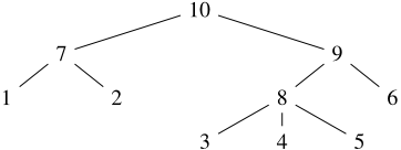
Example 3. Considering the criteria in Example 1, Fig. 1 depicts a criteria hierarchy aggregating the 6 initial critera to form 3 intermediate criteria: Overall price (7), comfort (8), technical properties (9), that are themselves aggregated to form the root node (10) yielding the overall score. The value in each node is computed as the Choquet integral from its children node values.
Compared to models with a single aggregation, thereafter referred to as flat models, hierarchical models offer several advantages:
- Representation power: hierarchical models are strictly more representative than flat models;
- Sparsity: hierarchical models involve fewer parameters than flat ones (see Ex. 4); likewise, the grouping of criteria into a smaller number of intermediate ones makes it easier for the decision maker to interpret the model;
- Representation of domain knowledge: hierarchical models can be tailored to reflect pieces of expert knowledge and thus better fit the mental representation of the decision maker;
- Hierarchical structures can be inspected at different levels of detail: if the decision maker needs to better understand the value of a given intermediate criterion, they can look at the values on its children nodes and get a fine-grained explanation thereof [Labreuche and Fossier, 2018].
Example 4 (Example 1 cont.). As said, a flat CI model including n attributes involves 2n - 2 parameters. The hierarchical model depicted in Fig. 1 includes 3 intermediate nodes with 2 children nodes, involving 2 parameters each, and 1 intermediate node with 3 children nodes, involving 6 parameters; the total number of parameters is thus 12, to be compared to 26 - 2 = 62 parameters for the flat model.
Letting a hierarchical model be defined as a directed rooted tree T with leaves L = {ℓi | i ∈ N} and a set of nonleaf nodes G, the set of children of g ∈ G is denoted by Ch(g) ⊆ G ∪ L, with Ch(g) ̸= ∅. Let fuzzy measure µg (resp. a marginal utility function ui) be associated with each node g (respectively, each leaf ℓi). The score so of each node o is computed recursively as follows:
- so(x) = ui(xi) if o ∈ L
- so(x) = Cµo ((sc(x) | c ∈ Ch(o))) if o ∈ g
The global score is sR(x) with R the root of T .
2.4 RelatedWork
MCDM models are commonly specified by marginal utility functions, aggregated through e.g. Choquet integrals. Thus, a (continuous or ordinal) utility score can be associated with each alternative, and different alternatives can be ranked based on these utilities. Current approaches focus on optimizing, eliciting or learning a single (flat) Choquet integral based on suitable training examples.
In constraint-based approaches, each training instance imposes a constraint on the sought utility model. [Grabisch et al., 2008] determine the fuzzy measures and their parameters complying with all these constraints. In [Benabbou et al., 2017], the constraint approach is extended and a min-max regret optimization problem is defined to gradually acquire the most informative constraints in the spirit of active learning approaches. The main limitation of the approach is its inability to deal with noisy and/or inconsistent training samples, possibly preventing the constraint problem from being satisfiable.
Based on a set of alternatives and the associated utilities, [Grabisch, 1995; Alavi et al., 2009] tackle the identification of a fuzzy measure as a supervised statistical learning problem, using gradient descent to optimize a logistic regression model, and using additional constraints to ensure that the solution defines a proper fuzzy measure (e.g., satisfies monotonicity). Along the same line, logistic regression is extended to learn Choquet integrals along a binary classification or ranking setting [Fallah Tehrani et al., 2012].
More recently, these methods are generalized to nonmonotonic fuzzy measures in [Havens and Anderson, 2018]. Finally, [Bourdache et al., 2019] use Bayesian linear regression to find the model parameters of e.g. 2-additive Choquet integrals or ordered weighted averages.
In the Additive Utility framework, [Bous and Pirlot, 2013] propose a probabilistic approach for learning the marginal utility functions of an additive utility model (a special case of the CI with marginal utilities). While other approaches to learning the Choquet integral assume marginal utility functions to be given, Choquistic Utilitaristic Regression (CUR) learns the aggregation and the marginal utilities simultaneously [Fallah Tehrani et al., 2014]. The associated (non convex) optimization problem is solved using a quadraticprogramming solver.
A method for learning hierarchical aggregation models, called fuzzy pattern trees, is proposed in [Huang et al., 2008; Senge and H¨ullermeier, 2011], using generalized averaging functions and/or triangular norms or co-norms as aggregation functions.
In [Senge and H¨ullermeier, 2015], the averaging functions are realized in the form of Choquet integrals, restricted to binary hierarchical tree-structures.
Discussion: The state of the art in (H)CI learning is restricted to either flat Choquet integrals 2 , or binary hierarchical tree-structure. NEUR-HCI ambitions to address these limitations by learning the parameterization of 2-additive HCI models together with marginal utilities in an efficient way, assuming that the hierarchical structure be given. As will be shown, NEUR-HCI satisfies by design the formal (e.g. monotonicity) or semantic (e.g. based on the expert hierarchy) constraints, thereby enforcing the soundness, interpretabiliy and semantic meaningfulness of the eventual model.
2 Furthermore these approaches, e.g. [Fallah Tehrani et al., 2012; Fallah Tehrani et al., 2014], hardly extend to HCI as they rely on a black-box sequential quadratic optimizer, and would face a nonconvex optimization problem in the hierarchical case.
3 ANeural Representation of Utilities
This section details how to jointly learn the marginal utilities and the parameters of their hierarchical aggregation, according to the tree-structure hierarchy provided by the expert. The difficulty is twofold: on the one hand, the underlying optimization problem is non-convex; on the other hand, the hierarchical structure of the aggregation makes it difficult to use a gradient-based approach 3 . Both difficulties are addressed by translating the sought model into a neural architecture, representing the marginal utilities and their aggregation through 2-additive Choquet integrals, and complying by design with their requirements. As said, only monotonic marginal utilities are considered in the following; the extension to more complex utilities is left for further work.
3.1 Representation of Marginal Utilities
A marginal utility ui : Xi ↦→ [0, 1] is a function mapping the i-th attribute domainXi to the unit interval. It is assumed that each domain 4 Xi to be set to R, and it is further assumed that the marginal utility ui increases with xi.
Marginal utility ui is represented as a weighted sum of sigmoids, as in [Fallah Tehrani et al., 2014]:
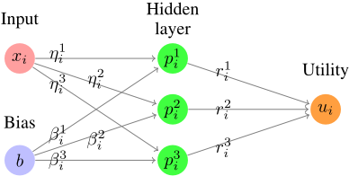
where hyper-parameter p sets the maximum number of sigmoids involved in the representation 5 ; βk i and ηk i respectively are the bias and precision parameters of the k-th sigmoid, and rk i its weight.
It is easy to see that ui satisfies the monotonicity and normalization constraints under the following conditions:
Accordingly, ui can be represented as a one hidden layer neural net (Fig. 2), involving p hidden neurons with sigmoidal activation function. Parameters η and r are clipped to 0 if they happen to become negative in the learning process; the fact that the r-values sum to one is ensured through batch normalization. This marginal utility, thereafter referred to as utility module, takes xi as input and returns utility ui(xi).
3.2 Representation of the Choquet Integral
As said, only 2-additive Choquet integrals are considered in the following, leaving the extension of the approach to kadditive integrals for future work. According to [Grabisch, 1997], a (flat) 2-additive Choquet integral on u = (u1 . . . un) can be written as follows:
3 An alternative would be offered by considering categorical variables, taking inspiration from e.g. [Jang et al., 2017].
4 In the case of a categorical attribute, e.g., color or name, ranging in {1, . . . ,m}, these values are ordered after the expert's preferences and mapped onto 1/m, 2/m, . . . , 1.
5 The actual number of sigmoids is minimized through L1 regularization, Eq. 10.
where ∧ and ∨ denote the min and max operators, respectively, and the weights wi, w∧ i,j , w∨ i,j are all non-negative and sum to one.
Most interestingly, the non-negativity constraints
are necessary and sufficient conditions to ensure that the 2additive Choquet integral is monotonous. The monotonicity property can thus be obtained through n2 constraints. Likewise, the constraint
is a necessary and sufficient condition to ensure the normalization of the Choquet integral. As shown below, these constraints can be enforced in a straightforward manner within the proposed neural architecture, making the representation of admissible utility functions and Choquet integrals significantly simpler.
Non-negativity constraints (Eq. 8) are enforced through a change of variables 6 . Formally, letting σ denote the differentiable softplus function, with σ(z) = ln(1 + exp(z)), then weight wi is sought as σ(zi) for some real-valued zi. Likewise, real-valued z∨ i,j (respectively z∧ i,j ) is introduced with w∨ i,j = σ(z∨ i,j ) (resp. w∧ i,j = σ(z∧ i,j )).
6 The option of clipping wi, w∧ i,j and w∨ i,j to 0 when they happen to become negative along the learning process, was discarded as it entailed a high instability of the trained model.
The normalization constraint (Eq. 9) is enforced through a batch normalization layer [Ioffe and Szegedy, 2015].
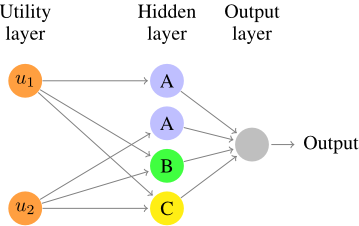
Overall, a 2-additive Choquet integral over an ndimensional utility vector u = (u1, . . . un), thereafter referred to as Choquet module, is represented as a neural architecture with a single hidden-layer with n2 neurons (Fig. 3), considering three types of neurons:
A : n neurons involve a single output ui and return wiui (with wi = σ(zi))
B : n(n-1) 2 neurons, denoted h∧i,j with inputs ui and uj, return σ(z∧ i,j ) × (ui ∧ uj) (corresponding to a weighted max-pooling on criteria i and j);
C : n(n-1) 2 neurons, denoted h∨i,j with inputs ui and uj, return σ(z∨ i,j ) × (ui ∨ uj) (corresponding to a weighted min-pooling on criteria i and j);
4 Learning the Hierarchical Choquet Integral
Building upon the above neural modules encoding marginal utility functions and 2-additive Choquet integrals, NEURHCI defines an neural architecture representing the overall hierarchical Choquet integral, combining marginal utilities according to the hierarchical tree structure of criteria aggregation provided by the expert. Back-propagation is leveraged to achieve the end-to-end learning of the overall neural net parameters, by exploiting the available data and optimizing a standard supervised learning criterion.
4.1 Neural Hierarchical Choquet Integral
Letting T denote the hierarchical aggregation structure on n criteria (Section 2.3), the target neural architecture is built by i/ creating a utility module C(ℓi) for each leaf ℓi and ii/ creating a Choquet module Cg for each node g ∈ G. The connection graph among the neural modules follows the tree structure of T , that is, the output of Cj for j ranging in Ch(g) form the input of Cg.
Example 5. The hierarchical Choquet integral described in Example 1 is implemented through 6 utility modules (one for each leaf) and 4 Choquet modules representing nodes 7, 8, 9 and 10, respectively, and denoted C7 (with input C1 and C2), C8 (with inputs C3, C4 and C5), C9 (with inputs C6 and C8) and finally C10 (with inputs C8 and C9).
Overall, the output of the neural net denoted C(x) depends on the weight vector concatenating the parameters of the utility and Choquet modules, denoted θ.
4.2 End-to-End Learning
The above neural architecture is trained using backpropagation, along three settings depending on the available dataset E.
Binary Classification In the simplest setting, E = {(x(j) , y(j) ), j = 1 . . .m}, where y(j) is the binary label associated to alternative x(j) ∈ X, indicating whether this alternative is good or bad. The neural net is trained using a standard classification criterion (e.g. cross-entropy) augmented with a L1 parsimony term aimed at minimizing the number of sigmoids in each marginal utility function:
with K the weight of the regularization term.
Regression Another setting is when E = {(x(j) , y(j) ), j = 1 . . .m} and y(j) ∈ [0, 1] is the real-valued utility of alternative x(j) . In this case, the neural net is trained using a standard regression criterion (e.g. mean squared error) augmented with a parsimony term as above:
Ranking A third setting is when E = {(x(j,1) , x(j,2) ), j = 1 . . .m} when the expert only indicates preferences x(j,1) ≻ x(j,2) between pairs of alternatives. The overall neural architecture is trained akin a Siamese network [Bromley et al., 1993; Burges et al., 2006]:
with A+ = max(A, 0), η a margin hyper-parameter (meant to enforce the fact that C(x(j,1) ) > C(x(j,2) ) + η, and K the weight of the parsimony term as above.
Discussion. Let us consider themodel spacemade of neural architectures, where each scalar input is passed through a utility module, the output of the utility modules are aggregated through a Choquet module, and the output of the Choquet modules are iteratively aggregated along other Choquet modules, following a tree-structure hierarchy T . By construction, this model space can represent any HCI-U (hierarchical Choquet Integral with utilities) when the number p of sigmoids goes to infinity [Cybenko, 1989]; furthermore, any model in this space is a valid HCI-U, satisfying monotonicity and normalization constraints by design. The identifiability issue, that is, whether the NEUR-HCI weight parameter θ is unique in the large sample limit, is left for further work.
5 Empirical Validation
This section reports on the empirical performance of NEURHCI comparatively to the state of the art.
5.1 Experimental Setting
The first goal of the experiments is to assess the robustness of NEUR-HCI along the classification, regression and ranking settings. The second goal is to investigate the respective impacts of learning marginal utilities and using a hierarchical aggregation. Accordingly, four NEUR-HCI variants have been considered: NCI learns a flat Choquet integral; NCI+U learns a flat CI together with marginal utilities; NHCI learns a hierarchical CI with a tree-structured hierarchy; NHCI+U learns an HCI together with marginal utilities.
NEUR-HCI variants are compared to the following baselines: Multilayer perceptron (MLP) with 1 fully connected hidden layer of n2 neurons, sigmoid activation function; Logistic regression (in the classification setting); Linear regression (in the regression and ranking settings); Choquistic Utilitaristic Regression 7 (CUR, in the classification setting) [Fallah Tehrani et al., 2014].
| Dataset | MLP | Logistic Reg. | CUR | NCI | NCI+U | NHCI | NHCI+U |
|---|---|---|---|---|---|---|---|
| CPU | 0.015 ± 0.021 | 0.091±0.051 | 0.024 ± 0.025 | 0.045±0.039 | 0.023±0.024 | 0.030±0.027 | 0.023±0.026 |
| CEV | 0.004 ± 0.004 | 0.110±0.023 | 0.084±0.067 | 0.059±0.012 | 0.051±0.023 | 0.035±0.009 | 0.019±0.017 |
| LEV | 0.135 ± 0.021 | 0.161± 0.022 | 0.143±0.0213 | 0.136 ± 0.022 | 0.135 ± 0.019 | N/A | N/A |
| MPG | 0.113 ± 0.036 | 0.090 ± 0.030 | 0.112 ± 0.099 | 0.086 ± 0.027 | 0.079 ± 0.027 | 0.085 ± 0.029 | 0.082 ± 0.027 |
| DB | 0.143 ± 0.069 | 0.164± 0.071 | 0.235 ± 0.017 | 0.139±0.067 | 0.132± 0.068 | 0.141 ± 0.068 | 0.135 ± 0.068 |
| MG | 0.179 ± 0.028 | 0.196 ± 0.027 | 0.166± 0.022 | 0.195 ± 0.027 | 0.166 ± 0.026 | 0.201 ± 0.030 | 0.191 ± 0.028 |
| Journal | 0.180 ±0.063 | 0.250±0.070 | 0.218±0.086 | 0.207±0.065 | 0.197±0.060 | 0.219±0.065 | 0.216±0.062 |
| Boston | 0.124 ± 0.030 | 0.145±0.033 | 0.1360± 0.085 | 0.127±0.031 | 0.129±0.032 | 0.121±0.032 | 0.129±0.031 |
| Titanic | 0.182 ± 0.025 | 0.202 ± 0.027 | 0.185 ± 0.041 | 0.192±0.0264 | 0.193 ± 0.027 | 0.203±0.027 | 0.194±0.027 |
| Dataset | MLP | Linear Reg. | NCI | NCI+U | NHCI | NHCI+U |
|---|---|---|---|---|---|---|
| CPU | 0.0005 ± 0.0016 | 0.0022±0.0019 | 0.0023±0.0032 | 0.0009±0.0013 | 0.0026±0.0023 | 0.0009±0.0011 |
| CEV | 0.0094 ± 0.003 | 0.0434±0.0442 | 0.0437±0.0037 | 0.0264±0.0027 | 0.0197±0.0017 | 0.0176±0.0017 |
| LEV | 0.0312 ± 0.0254 | 0.0252±0.0029 | 0.0252±0.0031 | 0.0252±0.0029 | N/A | N/A |
| MPG | 0.0047 ± 0.0008 | 0.0089±0.0019 | 0.0084±0.0018 | 0.0056±0.0013 | 0.0091±0.0018 | 0.0057±0.0012 |
| Journal | 0.0410 ± 0.010 | 0.0524±0.0128 | 0.0631±0.0127 | 0.0385±0.0112 | 0.0629 ± 0.0127 | 0.0391 ± 0.0117 |
| Boston | 0.0079 ± 0.0030 | 0.0174±0.0038 | 0.0157 ±0.0037 | 0.0072±0.0023 | 0.0151 ± 0.0033 | 0.0077 ± 0.0023 |
| Dataset | MLP | Linear Reg. | NCI | NCI+U | NHCI | NHCI+U |
|---|---|---|---|---|---|---|
| CPU | 0.0005 ± 0.002 | 0.0006 ± 0.003 | 0.0007 ± 0.003 | 0.0006 ± 0.003 | 0.0009 ± 0.003 | 0.0010 ± 0.004 |
| CEV | 0.0174 ± 0.012 | 0.0642±0.011 | 0.0243±0.005 | 0.0099±0.002 | 0.0165±0.004 | 0.0088±0.003 |
| LEV | 0.0178 ± 0.025 | 0.0179±0.023 | 0.0178 ±0.024 | 0.0177±0.023 | N/A | N/A |
| MPG | 0.0613 ± 0.012 | 0.0642±0.011 | 0.0610±0.011 | 0.0612±0.011 | 0.0633±0.012 | 0.0621±0.011 |
| DB | 0.1355 ± 0.0796 | 0.1257±0.079 | 0.1216±0.081 | 0.0942±0.069 | 0.1231 ± 0.092 | 0.0962 ± 0.081 |
| MG | 0.2601 ± 0.046 | 0.2661±0.047 | 0.2668±0.045 | 0.2381±0.037 | 0.2701±0.052 | 0.2446 ±0.036 |
| Journal | 0.1801 ± 0.064 | 0.1802±0.065 | 0.1761±0.063 | 0.1838±0.066 | 0.1711±0.063 | 0.1889±0.065 |
| Boston | 0.0659 ± 0.016 | 0.0790±0.014 | 0.0790±0.015 | 0.0669±0.012 | 0.0752 ± 0.014 | 0.0681 ± 0.014 |
| Titanic | 0.1521 ± 0.027 | 0.1651 ± 0.029 | 0.1632 ±0.028 | 0.1533 ±0.028 | 0.166 ± 0.028 | 0.1542 ± 0.029 |
| Arguments 1 | 0.0157 ± 0.015 | 0.0195±0.016 | 0.0145±0.012 | 0.0141±0.012 | 0.0141±0.012 | 0.0140±0.012 |
| Arguments 2 | 0.0588 ± 0.028 | 0.0653±0.031 | 0.0644±0.028 | 0.0581±0.027 | 0.0572±0.027 | 0.0572±0.028 |
| Arguments 3 | 0.0740 ± 0.039 | 0.0941±0.042 | 0.0783±0.040 | 0.0784±0.040 | 0.0761±0.039 | 0.0771±0.041 |
The standard MCDM benchmarks include CPU, CEV, LEV, MPG, DenBosch (DB), Mammographics (MG), Journal 8 , Boston Housing 9 , Titanic 10 and the Dagstuhl-15512 Arguments Quality corpus 11 [Wachsmuth et al., 2017]. The last one, reporting the preferences of three decision makers, yields three sub-datasets referred to as Arguments 1, Arguments 2, Arguments 3 (each one being associated with a single decision maker). A hierarchy is given for the CEV and Arguments datasets; for all other datasets but LEV, the authors managed to build a hierarchy; for LEV, no hierarchy was agreed upon (indicated as NA in the results). Overall, the number of features ranges from 4 to 15; the number of examples ranges from 119 to 1728. Ranking datasets are built from classification (respectively regression) datasets, setting that x(i) ≻ x(j) whenever y(i) > y(j) (resp. y(i) > y(j) + .05).
7 As the binarization used with CUR was not available, we ran CUR on the same splits and labels as NEUR-HCI for a fair comparison; this might explain the performance differences w.r.t. the original paper.
8 https://cs.uni-paderborn.de/?id=63916
9 http://lib.stat.cmu.edu/datasets/boston
10 https://web.stanford.edu/class/archive/cs/cs109/cs109.1166/ problem12.html
11 http://argumentation.bplaced.net/arguana/data
Each feature is associated with its monotonicity, i.e. whether the global score U(x) increases with xi 12 . All the features and labels in the training sets, were normalized linearly in [0, 1].
The performance indicators are measured as follows. Each dataset is randomly split into an 80% train and 20% test sets; the performance of the model trained from the train set is measured on the test set, and averaged over 1,000 random splits. Each time, all of the methods are evaluated on the same 1000 splits. Depending on the setting, the performance indicator is the misclassification rate, the mean squared error, and the swapping rate in the ranking setting.
12 The monotonicity is heuristically determined from the dataset, and decreasing criteria are multiplied by -1 to comply with the fact that a Choquet integral is non-decreasing w.r.t. its inputs.
NEUR-HCI hyper-parameters include the regularization weight K, set to 0 after a few preliminary experiments.
5.2 Analysis of the Results
Tables 1, 2 and 3 respectively report the NEUR-HCI performances in the classification, regression and ranking settings. The best result for each dataset is displayed in bold 13 . The MLP and NEUR-HCI computational costs are below 5 minutes for each dataset on an Intel i7. The CUR computational cost is not comparable (Matlab implementation).
As could have been expected, MLP generally behaves well; its number of weights, cubic in the number of criteria, however precludes the interpretation of the model. NEUR-HCI behaves on par or better than the other interpretable models, CUR and linear models.
A first remark is that learning marginal utilities does improve the performance: NCI+U and NHCI+U perform better than their NCI and NHCI counterparts. While this improvement can be naturally explained from the increased depth of the neural architecture and thus the higher complexity of the model, it does not come at the expense of the model interpretation.
A second remark is that hierarchical models outperform flat models on both datasets with an expert hierarchy (CEV and Arguments). On some other datasets, e.g. MPG, DG, MB, the hierarchy adversely affects the performance; as said, this hierarchy is merely guessed by the authors. This suggests that a flat model is preferable to one with an irrelevant hierarchy.
Most interestingly in terms of model identification, the solution trained from a given dataset along independent runs is very stable, i.e. the parameters always converge towards the same values 14 . Table 4 reports the variance over 100 runs of the 21 model parameters (the M¨obius representation [Grabisch and Labreuche, 2010]) on the CPU dataset. Further work will investigate the identifiability of the HCI within NEUR-HCI in the large sample limit.
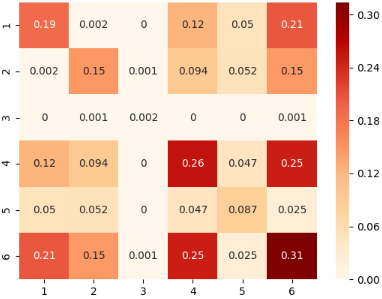
The model stability makes room for the easy visual inspection of the model. Indeed, a 2-additive model can be represented in the 2D plane, with the importance of the i-th criterion (respectively the synergy between i-th and j-th criteria) depicted as the color of the (i, i) (respectively (i, j) and (j, i)) squares: the darker the more important. As illustrated on Fig. 4, the most important criteria in the CEV domain are the safety rating (criterion 6) and to a lesser extent the passenger capacity (criterion 4); criteria 4 and 6 also happen to have a strong synergy. The buying price and the security rating also have a significant synergy. It is emphasized that this straightforward visualization enables the decision maker to instantly check the trained model; the estimated synergies can be confronted to the expectations and if needed the model can be revised by augmenting the dataset, adding samples to illustrate the desired effects.
13 when several results are in bold, this means that the difference is not statistically significant
14 A similar behavior is observed on artificial datasets, where NEUR-HCI exactly recovers the model used to label the data.
| 0.008±0.001 0.0±0.0 -0.007±0.006 0.03±0.011 0.121±0.006 0.047±0.005 0.08±0.006 | 0.008±0.002 0.016±0.006 0.001±0.001 0.168±0.008 0.025±0.008 -0.013±0.007 0.169±0.009 | 0.013±0.003 0.017±0.007 0.131±0.005 0.004±0.004 0.129±0.003 0.025±0.007 0.03±0.007 |
6 Conclusion and Perspectives
The NEUR-HCI framework presented in the paper relies on mapping a particular class of MCDM models, the 2additive hierarchical Choquet integrals, onto neural architectures. This original mapping relies on the definition of two elementary blocks: utility modules and Choquet modules. A 2-HCI with a given hierarchical aggregation structure T is mapped onto a neural net with a first layer made of utility modules, and other layers iteratively aggregating the criteria through Choquet modules according to T. The merit of the approach is twofold: on the one hand, the neural net complies by design with the 2-HCI constraints; on the other hand, its end-to-end training from data is achieved efficiently through back-propagation. The empirical validation of the approach demonstrates its good performance compared to other interpretable MCDMs, and the stability of the learned model.
The stability and interpretability of these models open some perspectives for further research in representation learning, as they enable to instantly confront the learned models with the expert expectations.
Future work will also consider the extension of the approach to 3-additive Choquet integrals, and aim to learn the aggregation tree structure from the data. Another research direction will investigate the identifiability of the 2-HCI.
@inproceedings{ijcai2020p275,
  title     = {Neural Representation and Learning of Hierarchical 2-additive Choquet Integrals},
  author    = {Bresson, Roman and Cohen, Johanne and Hüllermeier, Eyke and Labreuche, Christophe and Sebag, Michèle},
  booktitle = {Proceedings of the Twenty-Ninth International Joint Conference on
               Artificial Intelligence, {IJCAI-20}},
  publisher = {International Joint Conferences on Artificial Intelligence Organization},
  editor    = {Christian Bessiere},
  pages     = {1984--1991},
  year      = {2020},
  month     = {7},
  note      = {Main track},
  doi       = {10.24963/ijcai.2020/275},
  url       = {https://doi.org/10.24963/ijcai.2020/275},
}
TY - CPAPER TI - Neural Representation and Learning of Hierarchical 2-additive Choquet Integrals AU - Bresson, Roman AU - Cohen, Johanne AU - Hüllermeier, Eyke AU - Labreuche, Christophe AU - Sebag, Michèle T2 - Proceedings of the Twenty-Ninth International Joint Conference on Artificial Intelligence, IJCAI-20 PB - International Joint Conferences on Artificial Intelligence Organization PY - 2020 SP - 1984 EP - 1991 DO - 10.24963/ijcai.2020/275 UR - https://doi.org/10.24963/ijcai.2020/275 ER -Copied
Machine-readable versions of this paper, for tools and AI agents:





