
On Robustness in Qualitative Constraint Networks
Proceedings of the Twenty-Ninth International Joint Conference on Artificial Intelligence. Main track. Pages 1813-1819.
https://doi.org/10.24963/ijcai.2020/251
Keywords
- Knowledge Representation and Reasoning: Qualitative, Geometric, Spatial, Temporal Reasoning
Abstract
We introduce and study a notion of robustness in
Qualitative Constraint Networks (QCNs), which
are typically used to represent and reason about
abstract spatial and temporal information. In
particular, given a QCN, we are interested in obtaining
a robust qualitative solution, or, a robust scenario of
it, which is a satisfiable scenario that has a higher
perturbation tolerance than any other, or, in other
words, a satisfiable scenario that has more chances
than any other to remain valid after it is altered.
This challenging problem requires to consider the
entire set of satisfiable scenarios of a QCN, whose
size is usually exponential in the number of constraints
of that QCN; however, we present a first algorithm
that is able to compute a robust scenario of a QCN
using linear space in the number of constraints.
Preliminary results with a dataset from the
job-shop scheduling domain, and a standard one,
show the interest of our approach and highlight the
fact that not all solutions are created equal.
- [Allen, 1983] James F. Allen. Maintaining Knowledge about Temporal Intervals. Commun. ACM, 26:832-843, 1983.
- [Barber and Salido, 2015] Federico Barber and Miguel A. Salido. Robustness, stability, recoverability, and reliabil- ity in constraint satisfaction problems. Knowl. Inf. Syst., 44:719-734, 2015.
- [Barrett et al., 2016] Clark Barrett, Pascal Fontaine, and Ce- sare Tinelli. The Satisfiability Modulo Theories Library (SMT-LIB). www.SMT-LIB.org, 2016.
- [Bhatt et al., 2009] Mehul Bhatt, Frank Dylla, and Joana Hois. Spatio-terminological Inference for the Design of Ambient Environments. In COSIT, 2009.
- [Climent et al., 2010] Laura Climent, Miguel A. Salido, and Federico Barber. Robust Solutions in Changing Constraint Satisfaction Problems. In IEA/AIE, 2010.
- [Climent et al., 2014] Laura Climent, Richard J. Wallace, Miguel A. Salido, and Federico Barber. Robustness and Stability in Constraint Programming under Dynamism and Uncertainty. J. Artif. Intell. Res., 49:49-78, 2014.
- [Climent, 2015] Laura Climent. Robustness and stability in dynamic constraint satisfaction problems. Constraints, 20:502-503, 2015.
- [Cui et al., 1992] Zhan Cui, Anthony G. Cohn, and David A. Randell. Qualitative Simulation Based on a Logical For- malism of Space and Time. In AAAI, 1992.
- [Dylla and Wallgrün, 2007] Frank Dylla and Jan Oliver Wallgrün. Qualitative Spatial Reasoning with Conceptual Neighborhoods for Agent Control. J. Intell. Robotic Syst., 48:55-78, 2007.
- [Dylla et al., 2013] Frank Dylla, Till Mossakowski, Thomas Schneider, and Diedrich Wolter. Algebraic Properties of Qualitative Spatio-temporal Calculi. In COSIT, 2013.
- [Dylla et al., 2017] Frank Dylla, Jae Hee Lee, Till Mossakowski, Thomas Schneider, André van Delden, Jasper van de Ven, and Diedrich Wolter. A Survey of Qualitative Spatial and Temporal Calculi: Algebraic and Computational Properties. ACM Comput. Surv., 50:7:1-7:39, 2017.
- [Ginsberg et al., 1998] Matthew L. Ginsberg, Andrew J. Parkes, and Amitabha Roy. Supermodels and Robustness. In AAAI/IAAI, 1998.
- [Hebrard, 2007] Emmanuel Hebrard. Robust solutions for constraint satisfaction and optimisation under uncer- tainty. PhD thesis, University of New South Wales, Syd- ney, Australia, 2007.
- [Hirsch, 1999] Robin Hirsch. A Finite Relation Algebra with Undecidable Network Satisfaction Problem. Logic Jour- nal of the IGPL, 7:547-554, 1999.
- [Kostakis and Papapetrou, 2017] Orestis Kostakis and Pana- giotis Papapetrou. On searching and indexing sequences of temporal intervals. Data Min. Knowl. Discov., 31:809- 850, 2017.
- [Kostakis et al., 2017] Orestis Kostakis, Nikolaj Tatti, and Aristides Gionis. Discovering recurring activity in tempo- ral networks. Data Min. Knowl. Discov., 31:1840-1871, 2017.
- [Krishnaswamy et al., 2019] Nikhil Krishnaswamy, Scott Friedman, and James Pustejovsky. Combining Deep Learning and Qualitative Spatial Reasoning to Learn Com- plex Structures from Sparse Examples with Noise. In AAAI, 2019.
- [Ladkin and Reinefeld, 1992] Peter B. Ladkin and Alexan- der Reinefeld. Effective Solution of Qualitative Interval Constraint Problems. Artif. Intell., 57:105-124, 1992.
- [Ligozat and Renz, 2004] Gérard Ligozat and Jochen Renz. What Is a Qualitative Calculus? A General Framework. In PRICAI, 2004.
- [Ligozat, 2013] G. Ligozat. Qualitative Spatial and Tempo- ral Reasoning. ISTE. Wiley, 2013.
- [Liu and Li, 2012] Weiming Liu and Sanjiang Li. Solving Minimal Constraint Networks in Qualitative Spatial and Temporal Reasoning. In CP, 2012.
- [Moskovitch and Shahar, 2015] Robert Moskovitch and Yu- val Shahar. Classification of multivariate time series via temporal abstraction and time intervals mining. Knowl. Inf. Syst., 45:35-74, 2015.
- [Ragni and Wölfl, 2005] Marco Ragni and Stefan Wölfl. Temporalizing Spatial Calculi: On Generalized Neighbor- hood Graphs. In KI, 2005.
- [Suchan and Bhatt, 2016] Jakob Suchan and Mehul Bhatt. Semantic Question-Answering with Video and Eye- Tracking Data: AI Foundations for Human Visual Percep- tion Driven Cognitive Film Studies. In IJCAI, 2016. IJCAI
- [Suchan et al., 2018] Jakob Suchan, Mehul Bhatt, Przemys- law Andrzej Walega, and Carl P. L. Schultz. Visual Ex- planation by High-Level Abduction: On Answer-Set Pro- gramming Driven Reasoning About Moving Objects. In AAAI, 2018.
- [Suchan et al., 2019] Jakob Suchan, Mehul Bhatt, and Srikr- ishna Varadarajan. Out of Sight But Not Out of Mind: An Answer Set Programming Based Online Abduction Framework for Visual Sensemaking in Autonomous Driv- ing. In IJCAI, 2019. IJCAI
- [Verfaillie and Jussien, 2005] Gérard Verfaillie and Naren- dra Jussien. Constraint Solving in Uncertain and Dynamic Environments: A Survey. Constraints, 10:253-281, 2005.
- [Westphal and Wölfl, 2009] Matthias Westphal and Stefan Wölfl. Qualitative CSP, Finite CSP, and SAT: Compar- ing Methods for Qualitative Constraint-based Reasoning. In IJCAI, 2009. IJCAI
- [Wieland and Wallenburg, 2012] Andreas Wieland and Carl Marcus Wallenburg. Dealing with Supply Chain Risks: Linking Risk Management Practices and Strategies to Per- formance. Int. J. Phys. Distrib. Logist. Manag., 42:887- 905, 2012.
References were extracted automatically from the PDF and may contain errors.
Full text extracted automatically from the PDF; figures, tables and equations may differ. The PDF is the version of record.
1 Introduction
Qualitative Spatial and Temporal Reasoning (QSTR) is a major field of study in AI, and in particular in KR&R, that deals with the fundamental cognitive concepts of space and time in an abstract manner, via simple qualitative constraint languages [Ligozat, 2013; Dylla et al., 2017]. For instance, in natural language one uses qualitative expressions such as inside, before, and north of to spatially or temporally relate one object with another object or oneself, without resorting to providing quantitative information about these entities. Thus, QSTR provides a concise framework for rather inexpensive spatio-temporal reasoning and, hence, further boosts research to a plethora of application areas and domains, such as cognitive robotics [Dylla and Wallgr¨un, 2007], deep learning [Krishnaswamy et al., 2019], ambient intelligence [Bhatt et al., 2009], visual explanation [Suchan et al., 2018] and sensemaking [Suchan et al., 2019], semantic question-answering [Suchan and Bhatt, 2016], qualitative simulation [Cui et al., 1992], and spatio-temporal data mining [Moskovitch and Shahar, 2015; Kostakis and Papapetrou, 2017; Kostakis et al., 2017].
∗ Partially supported by Academy of Finland (#327352), National Natural Science Foundation of China (61806170), and Fundamental Research Funds for the Central Universities (2682018CX25).
Qualitative spatial or temporal information can be modeled as a Qualitative Constraint Network (QCN), which is defined as a network where the vertices correspond to spatial or temporal entities, and the arcs are labeled with qualitative spatial or temporal relations respectively. For instance x ≤ y can be a temporal QCN over Z. Given a QCN N, the literature is particularly interested in its satisfiability problem, which is the problem of deciding if there exists a spatial or temporal interpretation of the variables of N that satisfies its constraints, such an interpretation being called a solution of N. For instance, x = 0∧y = 1 is one of the (infinitely many) solutions of the aforementioned QCN, and x < y is the corresponding qualitative solution (satisfiable scenario) that concisely represents all the cases where x is assigned a lesser value than y. In general, for many widely adopted qualitative calculi the satisfiability problem is NP-complete [Dylla et al., 2013].
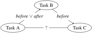
Motivation Let us consider the QCN of Figure 1, which, for the sake of our example, encodes the following scheduling problem: A factory produces a product that requires three tasks A, B, and C to be performed. Task B must be done before Task C, and Task A should take place either before or after B. As there might be unpredictable incidents concerning resource availability (e.g., power outage), how should the factory schedule production so that it may be least disturbed? In this case, if we choose the atom before as the preferred relation between Task A and Task B, then the only possible relation between Task A and Task C is before. However, if we place Task A after Task B, then we maintain the whole range of possibilities between Task A and Task C (e.g., before, during, after, or equals). In that way, whatever the change in the relation between Task A and Task C, any satisfiable scenario that places Task A after Task B, being more robust in comparison, will be able to maintain its satisfiability. In a sense, a robust scenario can be viewed as a satisfiable scenario of better quality than the rest, and as a proactive measure that limits as much as possible the need for successive repairs. Thus, it is an important notion in the context of uncertain and dynamic environments, such as real-life configurations.
Related work Robustness in the context of problem solving can probably be traced back to the introduction of search techniques for problem solving itself, as ever since there were ways to obtain solutions for a given problem, there was also a need to be able to differentiate between those solutions on some (usually robustness-related) basis; see for example [Ginsberg et al., 1998], and [Verfaillie and Jussien, 2005] and the references therein. Robustness has been studied quite extensively in the field of traditional constraint programming over the past years [Climent, 2015; Climent et al., 2014; Climent et al., 2010; Barber and Salido, 2015]. We note that in the aforementioned works notions related to robustness, such as stability, are studied as well, but these go beyond the scope of this paper. Briefly put, a solution is stable, if in the event of a change that invalidates it, it can be repaired with a minimum number of revisions, whereas a robust solution is more likely to remain valid after the change occurs; the distinction is subtle, but clear. To the best of our knowledge, robustness has not been studied at all in the context of infinite-domain CSPs, i.e., QCNs. Indeed, since a QCN has infinitely many solutions, as it is defined over an infinite domain such as space or time, comparing one solution against all others is an impossible task. Therefore, it is necessary to operate on a higher, symbolic, level and focus on qualitative solutions, i.e., satisfiable scenarios, instead. This suggests that the techniques that are used for CSPs cannot be readily applied to QCNs. (In support of the aforementioned statement, see also [Westphal and W¨olfl, 2009] for a comparison of various techniques for tackling QCNs.)
Contributions In this paper, (i) we introduce and study a notion of robustness in QCNs, and formally define the robustness problem and a robust scenario of a QCN, (ii) we present a first algorithm that is able to compute a robust scenario of a QCN using linear space in the number of constraints of that QCN, and that is modular in the sense that any state-of-the-art tool that is able to enumerate/generate satisfiable scenarios of a QCN can be employed during its execution, and (iii) we make a preliminary experimentation with a dataset from the job-shop scheduling domain, and a standard one, to assess the differences that exist between the scenarios of a given QCN.
2 Preliminaries
A binary qualitative constraint language is based on a finite set B of jointly exhaustive and pairwise disjoint relations, called the set of base relations (atoms), that is defined over an infinite domain D [Ligozat and Renz, 2004]. These base relations represent definite knowledge between two entities with respect to the level of granularity provided by the domain D; indefinite knowledge can be specified by a union of possible base relations, and is represented by the set containing them. The set B contains the identity relation Id, and is closed under the converse operation (-1 ). The entire set of relations 2B is equipped with the set-theoretic operations of union and intersection, the converse operation, and the weak composition operation denoted by ⋄ [Ligozat and Renz, 2004]. The weak composition (⋄) of two base relations b, b′ ∈ B is the smallest relation r ∈ 2B that includes b ◦ b′ ; formally, b ⋄ b′={b′′ ∈ B : b′′∩(b ◦ b′ ) ̸= ∅}, where b ◦ b′={(x, y) ∈ D × D : ∃z ∈ D such that (x, z) ∈ b ∧ (z, y) ∈ b′ }. Finally, for all r ∈ 2B , r-1 = ⋃{b-1 : b ∈ r}, and for all r, r′ ∈ 2B , r ⋄ r′ = ⋃{b ⋄ b′ : b ∈ r, b′ ∈ r′ }.
As an illustration, consider the well known qualitative temporal constraint language of Interval Algebra [Allen, 1983]. Its domain is defined to be the set of intervals on Q, i.e., D = {x = (x-, x+) ∈ Q × Q : x- < x+}. Then, each base relation can be defined by appropriately constraining the endpoints of two intervals, which yields a total of 13 base relations comprising the set B = {e, p, pi, m, mi, o, oi, s, si, d, di, f, fi}, as detailed in Figure 2. For example, d, viz., during, is defined as d = {(x, y) ∈ D × D : x- > y- and x+ < y+}. The identity relation Id of Interval Algebra is e, and its converse, i.e., e-1 , is defined to be again e.
The interested reader may find a detailed survey of qualitative spatial and temporal calculi in [Dylla et al., 2017].
The problem of representing and reasoning about qualitative spatial or temporal information can be tackled (among other ways) via the use of a Qualitative Constraint Network, defined in the following manner:
Definition 1. A qualitative constraint network (QCN) is a tuple (V, C) where:
- V = {v1, . . . , vn} is a non-empty finite set of variables, each representing an entity of an infinite domain D;
- and C is a mapping C : V × V → 2B such that C(v, v) = {Id} for all v ∈ V and C(v, v′ ) = C(v′ , v)-1 for all v, v′ ∈ V .
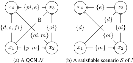
An example of a QCN is shown in Figure 2a; for clarity, neither converse relations nor Id loops are mentioned or shown in the figure, but they are part of any QCN.
Definition 2. Let N = (V,C) be a QCN, then:
- a solution of N is a mapping σ : V → D such that ∀v, v′ ∈ V , ∃b ∈ C(v, v′ ) such that (σ(v), σ(v′ )) ∈ b;
- N is satisfiable iff it admits a solution;
- N is trivially inconsistent, denoted by ∅ ∈ N, iff ∃v, v′ ∈ V such that C(v, v′ ) = ∅;
- N is the empty QCN on V , denoted by ⊥V , iff C(v, v′ ) = ∅ for all v, v′ ∈ V such that v ̸= v′ ;
- a sub-QCN N ′ of N, denoted by N ′ ⊆ N, is a QCN (V, C ′ ) such that C ′ (v, v′ ) ⊆ C(v, v′ ) ∀v, v′ ∈ V ;
- N is atomic iff ∀v, v′ ∈ V , C(v, v′ ) = {b} with b ∈ B;
- a scenario S of N is an atomic sub-QCN of N;
- the size of N, denoted by |N|, is |{(v, v′ ) : v, v′ ∈ V ∧ v < v′ }|.
In what follows, given some operation φ (such as the weak composition operation ⋄), the unique ⊆-maximal φconsistent sub-QCN of N is called the closure of N under φ-consistency and is denoted by φ(N).
We recall the definition of ⋄-consistency, which is a basic and widely used local consistency for reasoning with QCNs.
In the sequel, given a QCN N of some calculus, we assume that ⋄(N) always exists and that it is computable in polynomial time in |N|, and that ⋄-consistency decides the satisfiability of atomic QCNs. These assumptions hold for many widely adopted qualitative calculi [Dylla et al., 2013]; however, there do exist calculi (and new ones may arise) where the assumptions may not hold (e.g., [Hirsch, 1999]).
3 Robustness in QCNs
In this section, we introduce and study a notion of robustness in QCNs, and formally define related terms such as the robustness problem and a robust scenario of a QCN. Generally, robustness can be defined as "the ability of a system to resist change without adapting its initial stable configuration" [Wieland and Wallenburg, 2012]. In our context, we are interested in a satisfiable scenario of a QCN (see Figure 2b) with the ability to retain its satisfiability more than any other in the case where some of its constraints are changed. In other words, we are interested in obtaining a satisfiable scenario of a QCN that has more chances than any other to remain valid (satisfiable) after it is altered. We call such a scenario a robust scenario, a scenario with the maximum ability of resisting and avoiding unsatisfiability. Therefore, a robust scenario can be seen as a proactive measure that limits as much as possible the need for successive repairs, and hence can play an important role in environments that are prone to perturbation and unexpected change, such as real-life configurations.
Definition 4. (Perturbation) Given a QCN N and a scenario S of N, we say that S is perturbed iff one or more of its constraints change, resulting in a different scenario S ′ of N.
Before moving on to the main definitions of this section, we first introduce the operator #sameCons, which allows measuring the number of constraints that are the same respectively between two atomic QCNs over the same set of variables. More formally, given two atomic QCNs N = (V,C) and N ′ = (V, C ′ ), #sameCons(N,N ′ ) = |{(v, v′ ) : v, v′ ∈ V ∧ v < v′ ∧ C(v, v′ ) = C ′ (v, v′ )}|. We note that the condition v < v′ is used because C(v, v′ ) and C(v′ , v) concern a same constraint, since C(v, v′ ) = C(v′ , v)-1 for any QCN N = (V, C) and v, v′ ∈ V , and because C(v, v) = {Id} for any QCN N = (V, C) and v ∈ V .
In what follows, the set of scenarios of N will be denoted by [N] and the set of satisfiable scenarios of N by [[N]]. Clearly, for any given QCNN it holds that [[N]] ⊆ [N].
Next, we define a similarity measure to be able to assess how similar an atomic QCN N is on average to a set of atomic QCNs M (that may or may not include N ).
Definition 5. (SimilarityMeasure) Given an atomic QCNN and a set M of atomic QCNs over the same set of variables, the similarity measure of N with respect to M, denoted by similarity(N,M), is defined to be:
In other words, the similarity function with N and M as its parameters, measures the common constraints on average between N and each of the QCNs in M. Note that, for any given atomic QCN N and set M of atomic QCNs over the same set of variables, we have that:
Thereby, it is possible to use the similarity measure for atomic QCNs of different size.
Now, we define the notion of a robust scenario of a QCN.
Definition 6. (Robust Scenario) Given a QCNN, a scenario S of N is said to be robust iff we have that:
Intuitively, a robust scenario of a QCN N has the largest number of common constraints on average with each satisfiable scenario of N . To be in line with our claims in this paper, we assume that the following statistical property holds:
Property 1. Given a QCNN, the probability that a scenario S of N remains satisfiable once it is perturbed, is a monotonically increasing function of similarity(S, [[N]]).
Thus, a robust scenario of a QCN N is one that is more likely to fall within the set [[N]] when perturbed and, consequently, one that is more likely to withstand that perturbation.
Example 1. Let us view again the simplified QCN of Figure 1, and let us interpret it now as a QCN N of Interval Algebra (which has 13 base relations); so, before ∨ after becomes {p, pi}, before becomes {p}, and ? becomes B. A robust scenario S of N can be defined by labeling the arc between Task A and Task B with {pi}, and the arc between Task A and Task C with {p}. Then, S produces a similarity measure of around 0.7 when compared against the entire set [[N]] of 14 satisfiable scenarios of the QCN, which is the highest theoretically possible measure (as the measure is upper bounded by |N|+(|N|-1)·(|[[N]]|-1) |[[N ]]|·|N | , i.e., S must differ from any other scenario of [[N]] by at least one constraint). By contrast, a feeble scenario of N, when argmax is replaced by argmin in Definition 6, can be obtained by labeling the arc between Task A and Task B with {p}, and the arc between Task A and Task C with {p} (now the only possible option). This scenario produces a similarity measure of around 0.4.
The definition of the robustness problem of a QCN is straightforward.
Definition 7. (Robustness Problem) Given a QCNN, the robustness problem is finding a robust scenario S of N.
The robustness problem is an optimization problem; the related decision problem can be defined as follows:
Definition 8. (k-Robustness Problem) Given a QCN N and a rational number k ∈ [0, 1], the k-robustness problem is checking the existence of a scenario S of N such that S is satisfiable and we have that:
We have the following complexity result:
Proposition 1. Given a qualitative calculus Q for which the satisfiability problem is NP-complete, the k-robustness problem for Q is NP-hard.
Proof. We can solve the k-robustness problem of a given QCN N of Q by choosing k = 0 and determining if N is satisfiable. Hence, the k-robustness problem for Q is NP-hard as the satisfiability problem for Q is NP-hard.
Next, we formally define the notion of a maximum scenario of a QCN, which is not necessarily satisfiable:
Definition 9. (Maximum Scenario) Given a QCN N, a scenario S of N is said to be maximum iff we have that:
On its own, a maximum scenario of a given QCN can serve as a practical upper bound of the similarity measure that we can achieve. However, as [[N]] ⊆ [N], the following implied result (the detailed practical importance of which is unveiled in the next section) allows us to directly obtain a robust scenario of a QCN through a maximum scenario of it:
Proposition 2. Given a QCN N, a maximum scenario S of N is also a robust scenario of N iff S is satisfiable.
Finally, we end this section with the following result:
Proposition 3. Given a QCN N, a robust or maximum scenario of N is not unique in general.
Proof. Let us consider the QCN N = (V,C) that is defined by the variables v and v′ and the constraint C(v, v′ ) = {p, pi}. Each of its two scenarios is maximal and robust.
4 Algorithm for Robust Scenarios of QCNs
In this section, we present a first algorithm for obtaining a robust scenario of a QCN. Before doing so, let us briefly describe a naive algorithm for carrying out this task. Given a QCN N, a naive algorithm would compute the set [[N]] of satisfiable scenarios of N, and would then compare each one of those scenarios against all other. This would require O(|[[N]]|2 · |N| + |B||N| · α(N)) time and O(|N| · |[[N]]| + β(N)) space, where α(N) and β(N) would be the time and space needed respectively for obtaining a satisfiable scenario of N . The algorithm that we present in what follows is able to carry out the same task using O(|[[N]]| · |N|+|B||N| ·α(N))
Algorithm 1: RobustScen(N , Oracle)
in : A satisfiable QCN N = (V, C), and a generator Oracle that iterates [[N]]. out : A robust scenario of N. 1 begin 2 ν ← dict() 3 foreach v, v′ ∈ V : v < v′ do 4 ν[(v, v′ )] ← dict(); 5 foreach b ∈ B do 6 ν[(v, v′ )][b] ← 0; 7 foreach (V, C′ ) ∈ Oracle(N) do 8 foreach v, v′ ∈ V : v < v′ do 9 extract b from C′ (v, v′ ) = {b}; 10 ν[(v, v′ )][b] ← ν[(v, v′ )][b] + 1; 11 Smaximum = (V,C′ ) ←⊥V ; 12 foreach v, v′ ∈ V : v < v′ do 13 countmax ← 0 ; 14 foreach b ∈ B do 15 if ν[(v, v′ )][b] > countmax then 16 countmax ← ν[(v, v′ )][b]; 17 brelmax ← b; 18 C′ (v, v′ ) ← {brelmax}; 19 C′ (v′ , v) ← {brelmax}-1 ; 20 if ∅ ̸∈ ⋄(Smaximum) then return Smaximum ; 21 summax ← 0; 22 foreach (V, C′ ) ∈ Oracle(N) do 23 sum ← 0; 24 foreach v, v′ ∈ V : v < v′ do 25 extract b from C′ (v, v′ ) = {b}; 26 sum ← sum + ν[(v, v′ )][b]; 27 if sum> summax then 28 summax ← sum; 29 Srobust ← (V, C′ ); 30 return Srobust ;Algorithm 2: GenScen(N )
time and O(|N|+β(N)) space. In the end, we show that the space complexity can be as low as O(|N|), i.e., linear in |N|.
Let us come back to our algorithm, called RobustScen and presented in Algorithm 1. RobustScen first initializes a counter to store the number of occurrences of each base relation for each constraint over the set of all satisfiable scenarios of a given QCN N. Then, it calculates a maximum scenario of N by choosing the most frequent base relation for each constraint. If this maximum scenario is satisfiable, then it returns it, as it is also a robust scenario of N by Proposition 2; otherwise, it proceeds to obtain a robust scenario of N by calculating the similarity between a satisfiable scenario of N and [[N]], via the efficient use of the aforementioned counter. We note that to obtain a space complexity of as low as O(|N|), the set [[N]] needs to be recalculated. 1 This makes Proposition 2 of particular practical importance, as this recalculation may be avoided by simply checking if the obtained maximum scenario of N is satisfiable; such a check takes polynomial time in |N| (see Section 2). Finally, RobustScen receives as input a generator too, viz., Oracle, that iterates [[N]]; such a generator is presented in Algorithm 2. Simply put, a generator is a function that can stop midway (via the execution of the yield operator) and then continue from where it stopped.
Theorem 1. Given a satisfiable QCN N and a generator Oracle that iterates [[N]], Algorithm 1 returns a robust scenario of N using O(|[[N]]| · |N| + |B||N| · α(N)) time and O(|N |+β(N)) space, where α(N) and β(N) is the time and space needed respectively for the used generator to obtain a satisfiable scenario of N .
Proof. First, we prove that the output of the algorithm is a robust scenario of N. In lines 11-19, a scenario Smaximum = (V,C ′ ) is constructed in such a way that ∀v, v′ ∈ V the constraint C ′ (v, v′ ) is defined by a base relation b such that:
This implies that:
And finally by Definition 5 we obtain that:
Therefore, by Definition 9, Smaximum is a maximum scenario of N. In line 20, Smaximum is returned if it is satisfiable; hence, by Proposition 2 a robust scenario of N is returned.
In lines 21-29, a scenario Srobust is chosen such that:
By definition of the #sameCons operator, this can be rewritten as:
1 Even if we unify the satisfiable scenarios from the first calculation into the, so called, minimal sub-QCN of the input QCN [Liu and Li, 2012], extracting a scenario from that minimal sub-QCN is not any easier than extracting a scenario from the original QCN [Liu and Li, 2012]; we have also found this to be true in practice.
And finally by Definition 5 we obtain that:
Therefore, by Definition 6, Srobust is a robust scenario of N; hence, a robust scenario of N is returned in line 30.
Now, we prove the complexity of the algorithm. In lines 26, a dictionary (hash map) is constructed to count the frequency that a given base relation defines a constraint among all satisfiable scenarios. This takes O(|N|) time and space. Then, in lines 7-10 this dictionary is updated by iterating [[N]] and the constraints of each scenario in [[N]]. This takes O(|[[N]]| · |N| + |B||N| · α(N)) time and O(|N| + β(N)) space. In lines 11-19 a scenario is constructed and updated, which takes O(|N|) time and space. Finally, in lines 22-29, we again iterate [[N]] and the constraints of each scenario in [[N ]]. Thus, Algorithm 1 uses O(|[[N ]]| · |N |+|B||N | ·α(N )) time and O(|N | + β(N)) space to provide an output.
Given the use of Algorithm 2, called GenScen, in place of Oracle for Algorithm 1, we can obtain the following result:
Corollary 1. Given a satisfiable QCN N and the generator GenScen, Algorithm 1 returns a robust scenario of N using O(|[[N ]]|·|N |+|B||N | ·α(N )) time and O(|N |) space, where α(N) is the time needed to compute ⋄(N).
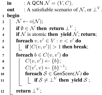
GenScen is an algorithmic representation of a recursive generator for iterating the satisfiable scenarios of a given QCN, which is based on the original algorithm described in [Allen, 1983] (also cf. [Ladkin and Reinefeld, 1992]).
5 Evaluation
In this section, we report on a preliminary experimentation that was performed primarily to assess the differences that may or may not exist between the scenarios of a given QCN N with respect to their similarity measure and perturbation tolerance. Secondarily, results are reported on the time needed to compute a robust scenario of N, on the size of [[N]], and on the % of the time that a maximum scenario of N is satisfiable and hence also a robust scenario of N.
Technical Specifications We used a computer with an Intel R© Xeon R© CPU E3-1231 v3 processor at 3.40GHz per core, 16 GB of RAM, and the Xenial Xerus x86 64 OS (Ubuntu Linux). All algorithms were coded in Python and run using PyPy 7.1.1. Only one CPU core was used.
Datasets We considered 100 satisfiable QCNs of 50 constraints each that were created using uniformly selected interval relations appearing in job-shop scheduling problems in the SMT-LIB [Barrett et al., 2016]; these QCNs involve relations from the set ˆB \ {{d, di, o, oi, s, si, f, fi, e}, {pi, mi, oi}, {p, m, o}} \ {{b} : b ∈ B}, where ˆB denotes the closure of B under intersection, weak composition, and converse. In addition, we considered 100 satisfiable QCNs of 50 constraints each that were created using uniformly selected standard interval relations, i.e., relations from 2B .
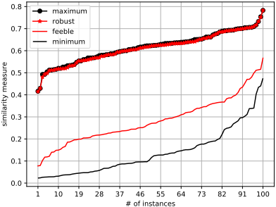
Results The results regarding the similarity measure of the various types of scenarios, viz., maximum, robust, feeble (when argmax is replaced by argmin in Definition 6), and minimum (when argmax is replaced by argmin in Definition 9) are depicted in Figure 3 for the dataset of job-shop interval relations. (The respective figure for the dataset of standard interval relations is qualitatively similar.) On average, the similarity measure for robust and feeble scenarios regarding job-shop interval relations is 0.61 and 0.28 respectively, i.e., a robust scenario is more than two times as robust as a feeble one. This ratio is even more pronounced regarding standard interval relations, as the similarity measure for robust and feeble scenarios in this case is 0.51 and 0.10 respectively on average, i.e., a robust scenario is more than five times as robust as a feeble one; this is likely due to the fact that 2B , being the entire set of interval relations, allows for more diverse constraints to be defined in general. In both cases, the similarity measure of a robust scenario is almost exactly the same as that of a maximum scenario. In fact, Table 1 shows that a maximum scenario is also a robust one around 50% of the time for both datasets used here, and also further strengthens our argument that using the set 2B of interval algebra relations allows for obtaining more diverse QCNs, which consequently yield more satisfiable scenarios.
| Dataset | |[[N]]| | %# ⏐↓maximum robust | time |
|---|---|---|---|
| Job-shop | 527573.53 | 45% | 4.70s |
| Standard | 896889.61 | 49% | 8.46s |
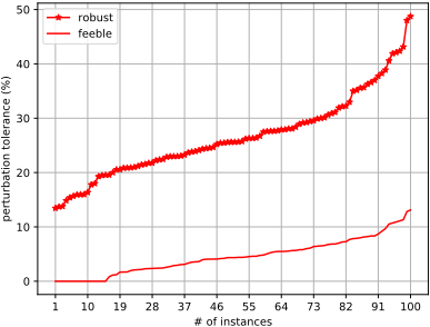
To obtain a first assessment of the perturbation tolerance of the various types of satisfiable scenarios, i.e., their ability to retain their satisfiability once they are perturbed, we computed for each considered scenario S all the possible perturbations that involved a change in a single constraint of S, and counted the times that S "survived" such a perturbation. In what follows, a perturbation tolerance of x% for a given satisfiable scenario suggests that the scenario was able to resist the aforementioned type of perturbation x% of the time. The results regarding the perturbation tolerance of robust and feeble scenarios are depicted in Figure 4 for the dataset of jobshop interval relations. (The respective figure for the dataset of standard interval relations is qualitatively similar.) We excluded maximum and minimum scenarios from the study as these are not necessarily satisfiable, and whenever they are they correspond to robust and feeble scenarios respectively (see Proposition 2). On average, the perturbation tolerance for robust and feeble scenarios regarding job-shop interval relations is 26.61% and 4.54% respectively, i.e., a robust scenario is almost six times more likely to withstand a perturbation than a feeble one. Regarding standard interval relations, the perturbation tolerance for robust and feeble scenarios is 20.73 and 1.15% respectively on average, i.e., a robust scenario is more than eighteen times more likely to withstand a perturbation than a feeble one.
6 Conclusion and FutureWork
In this paper, we introduced and studied a notion of robustness in QCNs, which are typically used to represent and reason about abstract spatial and temporal information in AI. In particular, given a QCN N, we investigated the problem of obtaining a robust scenario of N, which is a satisfiable scenario that has a higher perturbation tolerance than any other, or, in other words, a satisfiable scenario that has more chances than any other to remain valid after it is altered. Although this challenging problem typically requires to take into account the entire set of satisfiable scenarios of N, whose size is usually exponential in the number of its constraints, we presented here a first algorithm that computes a robust scenario of N using linear space in the number of constraints. Preliminary results with a dataset from the job-shop scheduling domain, and a standard one, show the interest of our approach and unveil vast differences among the scenarios of a QCN with respect to their robustness. Our work, being novel in QSTR, opens up many interesting directions of future work, from both a theoretical and a practical perspective. Computing a robust scenario of a QCN can be very costly, as our first computational bounds suggest, thus, it would be useful to define heuristics that would obtain a "good" scenario of a QCN in a more timely manner. Further, the related notions of stability and flexibility [Hebrard, 2007] would be worth exploring, and our current framework could be further extended with the integration of generalized neighborhood graphs that could be used to explicitly model allowed and/or disallowed perturbations [Ragni and W¨olfl, 2005]. Finally, it is an open question if the verification of a robust scenario is in NP.
@inproceedings{ijcai2020p251,
  title     = {On Robustness in Qualitative Constraint Networks},
  author    = {Sioutis, Michael and Long, Zhiguo and Janhunen, Tomi},
  booktitle = {Proceedings of the Twenty-Ninth International Joint Conference on
               Artificial Intelligence, {IJCAI-20}},
  publisher = {International Joint Conferences on Artificial Intelligence Organization},
  editor    = {Christian Bessiere},
  pages     = {1813--1819},
  year      = {2020},
  month     = {7},
  note      = {Main track},
  doi       = {10.24963/ijcai.2020/251},
  url       = {https://doi.org/10.24963/ijcai.2020/251},
}
TY - CPAPER TI - On Robustness in Qualitative Constraint Networks AU - Sioutis, Michael AU - Long, Zhiguo AU - Janhunen, Tomi T2 - Proceedings of the Twenty-Ninth International Joint Conference on Artificial Intelligence, IJCAI-20 PB - International Joint Conferences on Artificial Intelligence Organization PY - 2020 SP - 1813 EP - 1819 DO - 10.24963/ijcai.2020/251 UR - https://doi.org/10.24963/ijcai.2020/251 ER -Copied
Machine-readable versions of this paper, for tools and AI agents:





