Switch-List Representations in a Knowledge Compilation Map

1 Introduction

A Boolean function on n variables is a mapping from {0, 1}n to {0, 1}. There are many different ways in which a Boolean function may be represented. Common representations include truth table (TT), list of models (MODS), Boolean formulas (such as CNFs and DNFs), binary decision diagrams (BDDs, FBDDs, OBDDs), and negational normal forms (NNF, DNNF, d-DNNF). The task of transforming one representation of a given function f into another representation of f (e.g. transforming a DNF into an OBDD or a DNNF into a CNF) is called knowledge compilation. For a comprehensive review paper on knowledge compilation see [Darwiche and Marquis, 2002], where a Knowledge Compilation Map (KCM) is introduced. KCM systematically investigates different representation languages with respect to their relative succinctness, and the complexity of common transformations and queries.

In [Le Berre et al., 2018] the autors included PseudoBoolean constraint (PBC) and Cardinality constraint (CARD) languages into KCM by showing succinctness relations and the complexity of all queries and transformations introduced in [Darwiche and Marquis, 2002]. In this paper we aim at achieving exactly the same goal for the SL language.

Let f be a Boolean function with a fixed order of its n variables. The input binary vectors can be now thought of as binary numbers (with bits in the prescribed order) ranging from 0 to 2n - 1. An interval representation (IR) of f is then an abbreviated TT or MODS representation, where instead of writing out all the input vectors (binary numbers) with their function values, we write out only an ordered list of pairs [x, y] of integers, each pair specifying one interval of models. Interval representation of Boolean functions was introduced in [Schieber et al., 2005], where the input was considered to be a function f represented by a single interval (two n-bit numbers x, y) and the output was a DNF of f on n variables, i.e. a DNF which is true exactly on binary vectors (numbers) from the interval [x, y]. This knowledge compilation task originated from the field of automatic generation of test patterns for hardware verification [Lewin et al., 1995; Huang and Cheng, 1999].

In [ ˇCepek et al., 2008] the reverse knowledge compilation problemwas considered. Given a DNF, test if all models form a single interval under some permutation of variables, and in the affirmative case output the permutation and the two n-bit numbers defining the interval (note, that changing the order of variables may dramatically change the length of interval representations from O(n) to Ω(2n )). This problem is co-NP hard in general (it contains DNF tautology testing as a subproblem), but was shown to be poly-time solvable for tractable classes of DNFs (here tractable means that DNF falsifiability can be decided in poly-time). Recently, this result was extended to k-interval functions for arbitrary k (a function is k-interval if there exists a permutation of variables for which the interval representation consist of at most k intervals). The paper [ ˇCepek and Huˇsek, 2017] presents a recognition algorithm which runs in polynomial time in the length of the input DNF for any constant k (the complexity is exponential in k).

In fact, [ ˇCepek and Huˇsek, 2017] departs from interval representations and introduces switch-list representations which we shall use in this paper. A switch is a vector (binary number) x such that f(x-1) ̸= f(x). A switch-list is an ordered list of all switches of a given function. A switch-list of f together with the function value f(0) forms a switch-list representation (SLR) of f. It is important to keep the switch-lists ordered (instead of just keeping sets of switches) as this helps to keep the complexity of algorithms that work with SLR low.

SLR has an added advantage over interval representation, namely that a function and its negation have the same switchlists and the two representations differ only by the opposite values of f(0). The ease of taking a negation for SLR allows a trivial translation of any result relating SLR and DNF to a result relating SLR and CNF (and vice versa). For this reason, we shall use the SLR throughout this paper. It is not a limiting assumption in any way: clearly, an interval representation can be easily compiled in linear time to a SLR, and vice versa.

The language SL of all SLRs may be in some situations quite a good choice as a target compilation language. In the succinctness map SL is placed strictly above TT and MODS, incomparable to prime implicates (PI) and prime implicants (IP), and strictly below CNF, DNF, and OBDD languages. However, compared to CNF, DNF, and OBDD (and even IP and PI) the SL language has a wider set of supported queries and transformations.

SL supports all the queries from [Darwiche and Marquis, 2002] in poly-time, which is of course better than CNF and DNF languages but also better than IP and PI languages which do not support model counting. It is also better than the language of all OBDDs which do not support sentential entailment if the input OBDDs respect different orders of variables. The only language considered in [Darwiche and Marquis, 2002] with the same set of supported queries is the language of OBDDs with a fixed order of variables. Hence, the advantage of SL is, that it does not require the same order of variables for all inputs to guarantee poly-time performance for all queries. Moreover, an added advantage of SL lies in the computational simplicity of answering most queries - see Section 5 for details.

The biggest advantage of SL over the strictly more succinct languages such as CNF, DNF, and OBDD rests in the collection of supported transformations. SL supports negation in constant time (CNFs, DNFs, and MODS do not support negation in poly-time). SL also supports conditioning (but all common representations do, so this is not an advantage) and more importantly (general) forgetting which distinguishes it from OBDD. SL also supports unbounded conjunction and disjunction under the additional restriction that all input SLRs share the same set and order of variables. It should be noted here that OBDDs and even OBDDs with prescribed variable order fail to support unbounded conjunction and disjunction already in this restricted case. Of course, DNFs do not support unbounded conjunction, and CNFs do not support unbounded disjunction.

The collection of supported queries and transformations suggests that SL may be a very good choice in cases when many queries (such as model counting) have to be answered under many different additional assumptions such as partial substitution of binary values to subsets of variables (i.e. conditioning) or existential quantification of subsets of variables (i.e. forgetting). None of the above mentioned more succinct representations would support such a scenario in polynomial time. An obvious problem for this approach is a lack of compilation algorithms with SL as a target language. The only interesting example is the recognition algorithm from [ ˇCepek and Huˇsek, 2017], which may be in this context viewed as a compilation algorithm from tractable classes of DNF into SL (and by symmetry from tractable classes of CNF into SL). Note that the algorithm has a parameter k on its input, and the compilation which runs in time exponential in k is successful if and only if there exists a target SLR with at most k switches. Another representation which is also easy to compile into SL are binary decision trees with a fixed order of variables on all branches. By traversing the leaves of such a tree from left to right one can easily construct a SLR of the given function.

This is a theory paper which establishes the properties of the SL language and places it in KCM. We hope that the proven properties of SL will motivate an interest to find other classes of CNF, DNF, OBDD, or other representations, which can be efficiently compiled into SL.

2 Definitions and Notation

A Boolean function f in n variables can be represented by a truth table, which is a list of all 2n vectors together with their function values. Rather then listing all vectors, one can list only models of f (all vectors x for which f(x) = 1). The language of all such representations of all Boolean functions is called MODS, and each list of models for a particular function is called a sentence of the MODS language. Similarly we can consider sentences of non-models (all vectors x for which f(x) = 0) which define the language ¬MODS.

Other languages considered in this paper are CNF (consisting of all CNF sentences on the set PS of all propositional variables), DNF (consisting of all DNF sentences), PI (CNF sentences consisting of all prime implicates of a given function), IP (DNF sentences consisting of all prime implicants), OBDD< (ordered binary decision diagrams that respect some fixed total order < on the set PS), and OBDD (all ordered binary decision diagrams). For precise definitions of these languages we refer the reader to [Darwiche and Marquis, 2002]). Two sentences (possibly from two different propositional languages) are called logically equivalent if they represent the same function. Let us now define the principal language of this paper.

Definition 1. Let < be a total order on the set PS of all propositional variables, let X ⊆ PS of size n, and let f be a Boolean function on variables from X. Consider vector x ∈ {0, 1}n where the bits of x correspond to the variables of X in the prescribed order <. Each such vector x can be in a natural way identified with a binary number from [0, 2n - 1], so for every x > 0 the vector x-1 is well defined. We call x ∈ {0, 1}n a switch of f with respect to <, if f(x - 1) ̸= f(x). The list of all switches of f with respect to < is called the switch-list of f with respect to <. The switch-list of f with respect to < together with the function value f(0) is called the switch-list representation (SLR) of f with respect to <.

A function is k-switch iff it has a SLR with respect to some ordering < with at most k switches. The set of SLRs of all functions with respect to any < forms the language SL.

Definition 2. A propositional language L is at least as succinct as a propositional language K (L ≤ K) if and only if there exists a polynomial p such that for every sentence α ∈ K there exists a logically equivalent sentence β ∈ L such that |β| ≤ p(|α|). If L ≤ K holds and K ≤ L does not (K ̸≤ L), we write L < K.

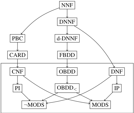
The diagram in Figure 1 summarizes the succinctness relations of many commonly used propositional languages. The main aim of the next section is to add the language SL into the framed part of the diagram in Figure 1.

3 Succinctness of Switch-list Representations

In this section we prove the succinctness relations for the SL language described in Figure 2.

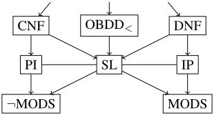
Proposition 3. CNF < SL and DNF < SL

Proof. Let us start by proving DNF ≤ SL. It was shown in [Schieber et al., 2005] that any 1-interval function (i.e. any function with at most two switches) on n variables can be compiled into a DNF with at most 2n - 4 terms, thus constructing an O(n2 ) size output for an O(n) size input. Now assume we have an SLR of function f with k switches on the input, which means that f has ⌊k/2⌋ or ⌊k/2⌋ + 1 intervals of models. By taking a disjunction of DNFs constructed for these individual intervals we get an O(kn2 ) size DNF representing f for an O(kn) size input. CNF ≤ SL follows by taking a negation both on the input and output.

SL ̸≤ DNF follows by contradiction from the fact that assuming SL ≤ DNF together with CNF ≤ SL would imply CNF ≤ DNF, which is known not to be true [Darwiche and Marquis, 2002]. The proof of SL ̸≤ CNF is symmetric.

Proposition 4. SL <MODS and SL < ¬MODS

Proof. The number of switches is clearly at most twice the number of models. On the other hand, function ∨ni=1 xi has one switch and 2n -1 models (similary for non-models).

The last strict succinctness relation in Figure 2 between SL and OBDD< is the most difficult to prove and requires several definitions and supporting lemmas.

Definition 5. Let f(x1, . . . , xn) be a Boolean function. A vector (y1, . . . , yl) ∈ {0, 1}l where l < n is called a relevant vector for f of length l if there exist two vectors (xl+1, . . . , xn), (x′l+1 , . . . , x′n ) ∈ {0, 1}n-l such that f(y1, . . . , yl, xl+1, . . . , xn) ̸= f(y1, . . . , yl, x′l+1 , . . . , x′n ).

Relevant vectors are prefix vectors (for the given order of variables) which are not sufficient for determining the value of f. The motivation behind the above definition is the easily verifiable fact that a k-switch function (i.e. a function which has k switches with respect to the prescribed order of variables) has at most k relevant vectors of any length.

Lemma 6. Let f(x1, . . . , xn) be a k-switch function and 1 ≤ l ≤ n an arbitrary number. Then there are at most k relevant vectors for f of length l.

Proof. Let yi = (yi1 , . . . , yin ), 1 ≤ i ≤ k be the switch vectors for f and let us assume these vectors are lexicographically ordered. That is ∀i ∈ {1, . . . , k - 1} : yi < yi+1 if we identify switch vectors with binary numbers. Consider the vectors pi = (yi1 , . . . , yi l ), 1 ≤ i ≤ k, that is the prefixes of the switch vectors of length l. There are at most k distinct vectors in this set as some pairs of prefixes may coincide. We claim that no other vector (different from p1 , . . . , pk ) is a relevant vector for f of length l. Let z = (z1, . . . , zl) be any such vector. Since z differs from all pi 's, there is no switch vector among vectors (z1, . . . , zl, xl+1, . . . , xn) for (xl+1, . . . , xn) ∈ {0, 1}n-l and thus

for any two vectors (xl+1, . . . , xn) ∈ {0, 1}n-l and (x′l+1 , . . . , x′n ) ∈ {0, 1}n-l , which proves that z is not relevant for f.

Remark 7. Note that in the above proof vectors p1 , . . . , pk are the only candidates for relevant vectors of length l, however not all of them have to be relevant for f, since the "decision" determining the value of f may be taken at an earlier index than l. A trivial example is a 1-switch function where f(0, x2, . . . , xn) = 0 and f(1, x2, . . . , xn) = 1 for all vectors (x2, . . . , xn). Here no (non-empty) prefix of the single switch vector (1, 0, 0, . . . , 0) is a relevant vector for f.

Definition 8. Let f(x1, . . . , xn) be a Boolean function. A relevant vector (y1, . . . , yl) for f of length l is called maximal relevant for f if neither (y1, . . . , yl, 0) nor (y1, . . . , yl, 1) are relevant vectors for f of length l + 1.

Lemma 9. Let f be a k-switch function. Then there are at most k maximal relevant vectors for f.

Proof. As we have seen in the proof of Lemma 6, only prefixes of the switch vectors are candidates to relevant vectors. Moreover for each switch vector at most one length of prefix can be a maximal relevant length, which proves the claim. (Note that for some switch vectors no prefix is relevant so there is also no maximal relevant prefix - see Remark 7.)

Lemma 10. Let f(x1, . . . , xn) be a Boolean function and let I ⊆ {x1, . . . , xn} be a subset of variables of size |I| = i. Let xm be the variable with the smallest index in I and let us assume that f has at most k maximal relevant vectors for f of length at least m. Then there are at most (ik +1) different Boolean functions that originate from f by fixing the values of variables in I.

Proof. If k = 0, that is there is no relevant vector for f of length m or larger, then f does not depend on variables from I. That means that all substitutions for the variables of I lead to the same function of (n - i) variables and the claim holds ((ik + 1) = (i · 0 + 1) = 1).

If k ≥ 1 we shall proceed by induction on |I| = i.

Base case (i = 1). By fixing the single variable in I to 0 or 1 we get at most two different functions of n - 1 variables, namely f(x1, . . . , xm-1, 0, xm+1, . . . , xn) and f(x1, . . . , xm-1, 1, xm+1, . . . , xn). Since i = 1 and k ≥ 1 we get ik + 1 ≥ 2 and the base case is verified.

Induction step. Let us assume that i > 1 and the statement of the lemma is true for 1, 2, . . . , i - 1. Let

be the set of all maximal relevant vectors for f of length at least m (by assumption l ≤ k). Consider the partition of V depending on the value of xm into

and denote |V0| = l0 and |V1| = l1. Clearly l0 + l1 = l.

Denote I ′ = I \ {xm} and let xm′ be the variable with the smallest index in I ′ (of course m′ > m). Consider functions of (n - 1) variables

There are at most l0 maximal relevant vectors for f0 of length at least m′ (and similarly for f1). Indeed, such maximal relevant vectors can originate from vectors in V0 (or V1 respectively) by deleting pim, if those vectors are long enough (have length at least m′ ). Thus we may use the induction hypothesis for f0, f1 and I ′ of size |I ′ | = i - 1. We get that

1. there are at most (i-1)l0+1 different Boolean functions originating from f0 by fixing the values of variables in I ′
2. there are at most (i-1)l1+1 different Boolean functions originating from f1 by fixing the values of variables in I ′

This altogether implies that there are at most

different Boolean functions that originate from f by fixing the values of variables in I, which finishes the proof.

Corollary 11. Let f(x1, . . . , xn) be a k-switch function and I ⊆ {x1, . . . , xn} a subset of its variables of size |I| = i. Then there are at most (ik + 1) different functions that originate from f by fixing variables in I.

Proof. This claim is a consequence of Lemmas 9 and 10.

Let us consider a k-switch function f(x1, . . . , xn), and let us consider an arbitrary reordering of the variables given by some linear order <. If we start branching on variables in the order given by <, then Corollary 11 states that after branching on the first i variables, we get at most (ik + 1) different Boolean functions of the remaining variables (as opposed to at most 2i for general functions). This is sufficient for a bound on the size of a minimal OBDD representation of f due to the following theorem.

Theorem 12 (3.2.2 [Wegener, 2000]). Let f be a function on variables X = {x1, . . . , xn} and let < be a linear order on X. Then the minimal-size OBDD representation of f respecting order < contains as many xi-nodes as there are different subfunctions |f|{xj|xj<xi}|.

Proposition 13. OBDD< < SL

Proof. Let f(x1, . . . , xn) be a k-switch function and < some linear order of the variables. By Theorem 12 and Corollary 11 a minimum size OBDD respecting < contains at most (ik+1) nodes on branching level i + 1 for 0 ≤ i ≤ n - 1. Therefore such an OBDD has at most ∑n-1 i=0 (ik+1) = 12 kn(n-1)+n nodes which is polynomial in the size of the input switch-list for f of size kn. This proves OBDD< ≤ SL.

On the other hand, it is easy to see that SL ̸≤ OBDD<, e.g. by considering the parity function.

The existential proof of Proposition 13 can be extended into a compilation algorithm, which for an input SLR of size kn outputs an OBDD of size O(kn2 ). This follows from the fact that conditioning (for any variable) can be done in polytime on a SLR (see Section 4), and so the output OBDD can be efficiently built level by level. The complexity bottleneck on each level is to check whether a node corresponding to a given subfunction already exists (in that case the algorithm just adds an arc to such a node) or not (in which case a new node must be created). If the SLRs for nodes on the current level (the one being built) are cached in an intelligent way to allow such equivalence checks, the overall complexity of the compilation algorithm can be bounded by O(k2n3 ).

To close this section, let us study the last missing succinctness relation in Figure 2.

Proposition 14. SL is incomparable with both PI and IP

Proof. SL ̸≤ PI (SL ̸≤ IP) follows from the fact that SL ≤ PI (SL ≤ IP) and OBDD ≤ SL (proved in Proposition 13) would imply OBDD ≤ PI (OBDD ≤ IP) which are both known not to be true [Darwiche and Marquis, 2002]. To show PI ̸≤ SL consider f on 2n variables x1, ..., xn and y1, ..., yn. The models of f are vectors {vi|i = 1, ..., n} where vi assigns only variables xi and yi to 1, and all other variables to 0. Thus f has exactly n models and the size of its SLR is O(n2 ) regardless of the order of variables. On the other hand, for an arbitrary subset of indices S ⊆ {1, ..., n} clause CS = (∨i∈S xi ∨ ∨i/∈S yi) is a prime implicate of f, and therefore f has at least 2n prime implicates, showing the claim. IP ̸≤ SL follows by symmetry.

Note, that function f from the proof of Proposition 14 has an exponential number of prime implicates with respect to the number of models, so PI ̸≤ MODS. Since MODS ̸≤ PI is trivial, this gives a short proof of the long standing open problem from [Darwiche and Marquis, 2002].

Corollary 15. PI is incomparable withMODS

4 Transformations

Transformations from [Darwiche and Marquis, 2002] include negation (¬C), bounded (∧BC) and unbounded (∧C) conjunction, bounded (∨BC) and unbounded (∨C) disjunction, conditioning (CD), singleton forgetting (SFO), and forgetting (FO). We also consider ∧C∗ and ∨C∗ which assume that all input SLRs are defined on the same set of variables and respect the same order of these variables, see Table 1.

Table 1: Transformations for the SL language, where ✓means the existence of a poly-time algorithm and ⋄ ∈ {∧, ∨}.

¬C: SLR can be trivially negated in constant time.

∧C∗ : Let f and g be two SLRs defined on the same set of variables and respectingthe same order of variables (the switches in both SLRs are vectors of the same length with coordinates indexed by the same variables). Observe that if x is neither a switch of f nor a switch of g it cannot be a switch of f ∧ g. Hence the SLR of f ∧ g is a subset of the union of the two input SLRs. Since both input SLRs are ordered, they can be easily merged into an ordered list and during the merge each switch can be checked whether it is a switch of f ∧ g or not. This can be done in linear time in the size of the input, and moreover this idea can be easily extended to any number of conjuncts and hence to the unbounded case. It is interesting to note that neither OBDD< nor OBDD languages support ∧C∗ [Darwiche and Marquis, 2002].

∧BC and ∧C: If SLRs f and g have different order of variables and/or different sets of variables, then the complexity of constructing a SLR of f ∧ g remains open.

∨C∗ , ∨BC, ∨C: The complexity status for disjunctions is the same as for conjunctions due to constant time negation.

CD: Let f be a function on variables x1, . . . , xn and let xi be an arbitrary variable. We interpret an assignment of variables x1, . . . , xi-1 as a binary number ℓ, 0 ≤ ℓ ≤ 2i-1 - 1, and denote the corresponding block of consecutive vectors sharing the same prefix ℓ in the truth table of f as Bℓ. Furthermore, we split Bℓ into B0 ℓ and B1 ℓ depending on the value of xi. We shall show how the SLR of f1 = f|xi=1 can be obtained from the SLR of f by a single pass through the input switch-list (the process for f0 = f|xi=0 is similar). We will write the vectors from the truth table of f as triples (ℓ, ∗, q) where ∗ ∈ {0, 1} represents the value of xi and 0 ≤ q ≤ 2n-i - 1 = 1 is a binary number representing xi+1, . . . , xn. Similarly, we will write the vectors from the truth table of f1 as pairs (ℓ, q).

When processing a switch of the type (ℓ, 0, q) we just count the parity p of the number of switches having the same prefix (ℓ, 0), i.e. the parity of the number of switches in the block B0 ℓ . After we pass the last switch in B0 ℓ , let us inspect the next switch in the list. If it differs from s = (ℓ, 1, 0) (the first vector in B1 ℓ ), p is odd, and ℓ > 0, we output s′ = (ℓ, 0). In this case s′ which originates from s by removing the xi coordinate becomes a switch of f1, replacing the odd number of switches in B0 ℓ . This is because f1(s′ ) = f(s) differs from f1(ℓ - 1, 1) = f(ℓ - 1, 1, 1). Note that (ℓ - 1, 1, 1) is the last vector in B1 ℓ-1 and so (ℓ - 1, 1) is a predecessor of s′ in the truth table of f1. If p is even or ℓ = 0, then the switches in B0 ℓ "disappear" without creating any switch for f1.

When processing a switch of the type s = (ℓ, 1, q) where q > 0 we simply output s′ = (ℓ, q) (all such switches of course "survive" the conditioning xi = 1). If s = (ℓ, 1, 0) (switch s is the first vector in B1 ℓ ), we output s′ = (ℓ, 0) only if p obtained from B0 ℓ is even (this includes the case if there are no switches in B0 ℓ ) and ℓ > 0. Clearly, also in this case s′ is indeed a switch of f1 because its function value differs from the last vector in B1 ℓ-1 which becomes its predecessor in the truth table of f1. On the other hand, if p is odd or ℓ = 0 then s "disappears" without creating a switch for f1.

If the input SLR has k switches, the above described process of conditioning on xi takes O(n) time per switch (and each switch is processed exactly once), and therefore can be implemented to run in O(kn) time. Since the output SLR has at most as many switches as the input SLR, we can repeat the process |S| times to achieve conditioning on any set S of variables in O(kn2 ) time. However, the O(kn) time complexity can be maintained even in this case. If we divide the truth table of f into blocks with respect to the least significant variable in S (the rightmost one in the truth table), then instead of the alternating pattern of disappearing and surviving blocks for |S| = 1 (as described above) we get a pattern of possibly many disappearing blocks followed by a single surviving block. However, the idea of conditioning can remain the same. We count the parity of the number of switches in between two surviving blocks, treat the first vector in the next surviving block accordingly, then output the remaining switches in the surviving block.

SFO and FO: Let f be a function on variables x1, . . . , xn and let xi be an arbitrary variable. We shall show how the SLR of fi = ∃xif can be obtained from the SLR of f in polynomial time. The procedure can be implemented directly on SLRs, but we find it more understandable if explained on interval representations (IRs) which actually motivated the introduction of SLRs. We first compile the SLR of f into an IR of f, then transform this into an IR of fi, and finally compile back into an SLR of fi. The first and third steps take linear time, so it remains to describe the second step. We again (as for CD) consider the block structure Bℓ = B0 ℓ ∪B1 ℓ for 0 ≤ ℓ ≤ 2i-1 - 1 of the truth table of f and also use the (ℓ, ∗, q) notation for the vectors from the truth table of f and (ℓ, q) for the vectors from the truth table of fi.

When passing through the ordered list of intervals in IR of f, an interval [a, b] is processed depending on whether a ∈ B0 ℓ or a ∈ B1 ℓ (for some ℓ) as follows. For a = (ℓ, 0, q) if

• (a) b = (ℓ, 0, r) output [(ℓ, q), (ℓ, r)],

On the other hand, for a = (ℓ, 1, q) if

• (e) b = (ℓ, 1, r) output [(ℓ, q), (ℓ, r)],

It is easy to check in each of the above seven cases that the models of f in the interval [a, b] really translate to models of fi in the specified output intervals. However, the output intervals may of course overlap (or even be identical, e.g. a pair of intervals obtained from (a) and (e) may be identical) so another "consolidation" pass through the output is necessary, which replaces any set of overlapping intervals with their union.

The above considerations imply that forgetting a single variable SFO can be performed in polynomial time. To see that the same is true for FO, we must analyze more carefully case (b), which is the only one when a single interval [a, b] of f may produce two intervals of fi. If it does, we will call [a, b] a splitting interval. Note that if q ≤ r, the two output intervals merge in the consolidation pass, so [a, b] = [(ℓ, 0, q), (ℓ, 1, r)] is splitting if and only if q > r. Hence q ̸= 0 and r ̸= 1 are necessary conditions for [a, b] = [(ℓ, 0, q), (ℓ, 1, r)] to be a splitting interval.

Observe also, that for a = (ℓ, ∗, 0) the interval [a, b] produces only such intervals [a′ , b′ ] where a′ = (ℓ, 0), and for b = (k, ∗, 1) the interval [a, b] produces only such intervals [a′ , b′ ] where b′ = (k, 1).

Putting the facts from the previous two paragraphs together implies, that if we forget the variables in the decreasing order of significance (most significant variables first), neither of the two intervals generated by a splitting interval [a, b] can become a splitting interval when forgetting subsequent variables. Indeed, either the suffix of the left margin of the generated interval is all zeros (and stays all zeros from then on in subsequent forgetting), or the suffix of the right margin of the generated interval is all ones (and stays all ones). Thus, forgetting any subset of variables may altogether at most double the number of intervals on the output, which implies that FO can be done in poly-time by repeating SFO.

5 Queries

Standard queries from [Darwiche and Marquis, 2002] include consistency (CO), validity (VA), implicant check (IM), clausal entailment (CE) , sentential entailment (SE), equivalence check (EQ), model counting (CT), and model enumeration (ME). Since all these queries can be answered in poly-time for the OBDD< language, the same is true for SL which can be compiled into OBDD< in poly-time (see Section 3).

It is clear that for most queries direct algorithms using SLR are more efficient than indirect algorithms that first compile the input SLR into an OBDD. Obviously, CO and VA checks take constant time. If the input SLR has k switches, IM and CE can be implemented to run in O(kn) time using conditioning and a validity check. SLRs are also very well suited for model counting (O(k) subtractions on n-bit numbers suffice) and for model enumeration, which takes linear time w.r.t. the output size. Also SE and EQ take linear time if both inputs share the same set and order of variables as they can be answered using negation, disjunction, and validity check. The only queries that are expensive are SE and EQ in case the two inputs have different variable orders. We do not have direct algorithms that manipulate SLRs for these queries at the present moment, instead we compile both input SLRs into OBDDs (both respecting the same order of variables) and run the query algorithms for these OBDDs. Finding direct algorithms for SE and EQ which would avoid compilation into OBDDs may be a good research topic.

6 Conclusions

The main aim of this paper is to include the SL language into KCM [Darwiche and Marquis, 2002] and to argue that it may constitute a reasonable target language. This aim is justified by completing three subtasks: (1) derive the relative succinctness of SL compared to the languages already considered in [Darwiche and Marquis, 2002], (2) establish the complexity status of common transformations for SL, and (3) do the same for common queries. This goal is achieved with few open problems remaining, namely the complexity of conjunctions and disjunctions of SLRs on different sets of variables.

The results in this paper are crucially dependent on the chosen order of vectors in the truth table (the natural lexicographic order). There are other orders which are quite natural as well. For instance, one can order vectors based on the number of ones and complement this by some natural order on the sets of vectors with the same number of ones. Such a "cardinality" order has quite different properties, note that e.g. the parity function which has only exponentially large SLRs with respect to the lexicographic order of vectors has a linear size SLR with respect to the "cardinality" one. Examining the properties of SLRs with respect to non-standard orders of vectors may be the subject of a future study.

Acknowledgements

The authors gratefully acknowledge a support by the Czech Science Foundation (Grant 19-19463S).