
Simultaneous Arrival Matching for New Spatial Crowdsourcing Platforms
Proceedings of the Twenty-Ninth International Joint Conference on Artificial Intelligence. Main track. Pages 1279-1287.
https://doi.org/10.24963/ijcai.2020/178
Keywords
- Data Mining: Mining Spatial, Temporal Data
- Data Mining: Other
Abstract
In recent years, 3D spatial crowdsourcing platforms become popular, in which users and workers travel together to their assigned workplaces for services, such as InterestingSport and Nanguache. A typical problem over 3D spatial crowdsourcing platforms is to match users with suitable workers and workplaces. Existing studies all ignored that the workers and users assigned to the same workplace should arrive almost at the same time, which is very practical in the real world. Thus, in this paper, we propose a new Simultaneous Arrival Matching (SAM), which enables workers and users to arrive at their assigned workplace within a given tolerant time. We find that the new considered arriving time constraint breaks the monotonic additivity of the result set. Thus, it brings a large challenge in designing effective and efficient algorithms for the SAM. We design Sliding Window algorithm and Threshold Scanning algorithm to solve the SAM. We conduct the experiments on real and synthetic datasets, experimental results show the effectiveness and efficiency of our algorithms.
- [Bei and Zhang, 2018] Xiaohui Bei and Shengyu Zhang. Al- gorithms for trip-vehicle assignment in ride-sharing. In AAAI, pages 3-9, 2018.
- [Chen et al., 2014] Zhao Chen, Rui Fu, Ziyuan Zhao, Zheng Liu, Leihao Xia, Lei Chen, Peng Cheng, Caleb Chen Cao, Yongxin Tong, and Chen Jason Zhang. gmission: A gen- eral spatial crowdsourcing platform. PVLDB, 7(13):1629- 1632, 2014.
- [Chen et al., 2019] Zhao Chen, Peng Cheng, Yuxiang Zeng, and Lei Chen. Minimizing maximum delay of task as- signment in spatial crowdsourcing. In ICDE, pages 1454- 1465, 2019.
- [Cheng et al., 2015] Peng Cheng, Xiang Lian, Zhao Chen, Rui Fu, Lei Chen, Jinsong Han, and Jizhong Zhao. Re- liable diversity-based spatial crowdsourcing by moving workers. PVLDB, 8(10):1022-1033, 2015.
- [Cheng et al., 2017a] Peng Cheng, Xiang Lian, Lei Chen, and Cyrus Shahabi. Prediction-based task assignment in spatial crowdsourcing. In ICDE, pages 997-1008, 2017.
- [Cheng et al., 2017b] Yurong Cheng, Ye Yuan, Lei Chen, Christophe G. Giraud-Carrier, and Guoren Wang. Com- plex event-participant planning and its incremental variant. In ICDE, pages 859-870, 2017.
- [Cheng et al., 2018] Peng Cheng, Xun Jian, and Lei Chen. An experimental evaluation of task assignment in spatial crowdsourcing. PVLDB, 11(11):1428-1440, 2018.
- [Gale and Shapley, 2013] D. Gale and L. S. Shapley. College admissions and the stability of marriage. The American Mathematical Monthly, 120(5):386-391, 2013.
- [Gao et al., 2016] Dawei Gao, Yongxin Tong, Jieying She, Tianshu Song, Lei Chen, and Ke Xu. Top-k team rec- ommendation in spatial crowdsourcing. In WAIM, pages 191-204, 2016.
- [Karp et al., 1990] Richard M. Karp, Umesh V. Vazirani, and Vijay V. Vazirani. An optimal algorithm for on-line bipar- tite matching. In STOC, pages 352-358, 1990.
- [Kazemi and Shahabi, 2012] Leyla Kazemi and Cyrus Sha- habi. Geocrowd: enabling query answering with spatial crowdsourcing. In SIGSPATIAL, pages 189-198, 2012.
- [Li et al., 2019] Boyang Li, Yurong Cheng, Ye Yuan, Guoren Wang, and Lei Chen. Three-dimensional stable matching problem for spatial crowdsourcing platforms. In KDD, pages 1643-1653, 2019.
- [She et al., 2015] Jieying She, Yongxin Tong, and Lei Chen. Utility-aware social event-participant planning. In SIG- MOD, pages 1629-1643, 2015.
- [She et al., 2017] Jieying She, Yongxin Tong, Lei Chen, and Tianshu Song. Feedback-aware social event-participant ar- rangement. In SIGMOD, pages 851-865, 2017.
- [Song et al., 2017] Tianshu Song, Yongxin Tong, Libin Wang, Jieying She, Bin Yao, Lei Chen, and Ke Xu. Trichromatic online matching in real-time spatial crowd- sourcing. In ICDE, pages 1009-1020, 2017.
- [Song et al., 2018] Tianshu Song, Feng Zhu, and Ke Xu. Specialty-aware task assignment in spatial crowdsourcing. In AISC, pages 243-254, 2018.
- [Tao et al., 2018] Qian Tao, Yuxiang Zeng, Zimu Zhou, Y- ongxin Tong, Lei Chen, and Ke Xu. Multi-worker-aware task planning in real-time spatial crowdsourcing. In DAS- FAA, pages 301-317, 2018.
- [To et al., 2015] Hien To, Cyrus Shahabi, and Leyla Kaze- mi. A server-assigned spatial crowdsourcing framework. TSAS, 1(1):2:1-2:28, 2015.
- [Tong et al., 2016] Yongxin Tong, Jieying She, Bolin Ding, Lei Chen, Tianyu Wo, and Ke Xu. Online minimum matching in real-time spatial data: Experiments and anal- ysis. PVLDB, 9(12):1053-1064, 2016.
- [Tong et al., 2017] Yongxin Tong, Libin Wang, Zimu Zhou, Bolin Ding, Lei Chen, Jieping Ye, and Ke Xu. Flexible online task assignment in real-time spatial data. PVLDB, 10(11):1334-1345, 2017.
- [Tong et al., 2018a] Yongxin Tong, Libin Wang, Zimu Zhou, Lei Chen, Bowen Du, and Jieping Ye. Dynamic pricing in spatial crowdsourcing: A matching-based approach. In SIGMOD, pages 773-788, 2018.
- [Tong et al., 2018b] Yongxin Tong, Yuxiang Zeng, Zimu Zhou, Lei Chen, Jieping Ye, and Ke Xu. A unified ap- proach to route planning for shared mobility. PVLDB, 11(11):1633-1646, 2018.
- [Tran et al., 2018] Luan Tran, Hien To, Liyue Fan, and Cyrus Shahabi. A real-time framework for task as- signment in hyperlocal spatial crowdsourcing. TIST, 9(3):37:1-37:26, 2018.
- [Xia et al., 2019] Jinfu Xia, Yan Zhao, Guanfeng Liu, Jia- jie Xu, Min Zhang, and Kai Zheng. Profit-driven task as- signment in spatial crowdsourcing. In IJCAI, pages 1914- 1920, 2019. IJCAI
- [Zhao et al., 2019a] Boming Zhao, Pan Xu, Yexuan Shi, Y- ongxin Tong, Zimu Zhou, and Yuxiang Zeng. Preference- aware task assignment in on-demand taxi dispatching: An online stable matching approach. In AAAI, pages 2245- 2252, 2019.
- [Zhao et al., 2019b] Yan Zhao, Jinfu Xia, Guanfeng Li- u, Han Su, Defu Lian, Shuo Shang, and Kai Zheng. Preference-aware task assignment in spatial crowdsourc- ing. In AAAI, pages 2629-2636, 2019.
References were extracted automatically from the PDF and may contain errors.
Full text extracted automatically from the PDF; figures, tables and equations may differ. The PDF is the version of record.
1 Introduction
In recent years, with the development of Internet and mobile service, spatial crowdsourcing platforms show their popularity in people's daily life and attract much attention of researchers. In spatial crowdsourcing platforms, assigning tasks to suitable workers is one of the core issues [Chen et al., 2019][Cheng et al., 2015][Cheng et al., 2017a] [Cheng et al., 2018][Song et al., 2018][Bei and Zhang, 2018] [Tran et al., 2018][Tong et al., 2018a][Tao et al., 2018] and have achieved good results in 2D platforms. However, the emerging of 3D platforms, such as sport-training platforms 1 and customer-makeup platforms 2 , bring new challenges. On 3D platforms, users and workers are required to travel together to their assigned workplace for services. For example, on the Nanguache platform 2 , a customer and his/er assigned hairdresser would go together to an arranged barbershop for a haircut. The 2D matching methods cannot solve the matching requests for 3D platforms, and thus Song et al. [Song et al., 2017] proposed a 3D matching as a consequence, calculating the online matching of users, workers and workplaces. However, such 3D matching failed to consider the service preference of users and workers. Thus, Li et al. [Li et al., 2019] proposed a 3D stable matching. It can make sure that no matched workers and users both prefer a second workplace to the matched one.
∗Contact Author
1 http://www.quyundong.com/.
2 http://www.nanguache.com/.
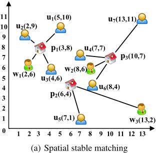
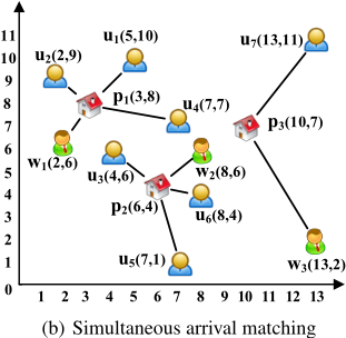
Unfortunately, all the above existing studies ignored an important factor that the workers and users matched to the same workplace should arrive almost at the same time. For example, Fig. 1 shows 3 workers (w1-w3), 7 users (u1-u7) and 3 workplaces (p1-p3) on a platform. The capacity of each worker is {3, 3, 1} respectively, which shows the maximum number of users s/he can serve. The matching result obtained from [Li et al., 2019] is shown in Fig. 1(a). However, in the real world, each user and worker has a departure time, which means the time they wish to leave their current location for their workplace. And it will take them some time to travel to the target workplaces. Suppose the departure time is shown in Table 1 and the travel speed of each user and worker is 0.5. Then u5 departs at 9:05 and reaches p2 at 9:12. According to the result in Fig. 1(a), w3 reaches p2 at 9:24, which means that u5 should wait w3 for 12 minutes. Similarly, u4 reaches p3 at 9:08 and he needs to wait for u7 until 9:30. Neither u4 nor u5 will be happy.
Motivated by the above example, we propose a new model which ensures that the workers and users reach their matched workplace within a given tolerant time. We call such matching as a Simultaneous Arrival Matching (SAM) problem. Nevertheless, in the matching of the existing work [Song et al., 2017], there also exists an arriving time and a leaving time for each worker and user. In their work, the arriving time means when each user and worker is available, and they should be matched (i.e., responded by the platform) before their leaving time. The period between each arriving time and leaving time is the maximum response time of each worker's or user's request. Their arriving time and leaving time have different meanings compared with ours, and they did not consider when each matched user and worker would arrive at their assigned workplace. Since considering such constraint on arriving time breaks the monotonic additivity of the matching results (detailed in Theorem 3 in Section 2), it brings a large challenge of existing approaches to solve SAM effectively and efficiently. We prove that the SAM problem is NPhard and the monotonic additivity of the matching results. We present two approximate algorithms to solve it. In summary, we make the following contributions.
| 9:01 | 9:02 | 9:03 | 9:04 | 9:05 | 9:06 | 9:07 | 9:08 | 9:09 | 9:10 |
| u4 | u1 | u2 | w1 | u5 | w2 | u6 | u3 | w3 | u7 |
- We propose a new stable matching problem called Simultaneous Arrival Matching (SAM) enabling users and workers arriving at their assigned workplace nearly at the same time. We prove that the matching results of SAM have no monotonic additivity.
- We devise a greedy algorithm, named Sliding Window. It greedily matches workers according to their capacity, and utilizes the arriving order of users and the waiting time constraint to prune the number of candidate users.
- In order to improve the effectiveness and make the algorithm as efficient as possible, we propose a thresholdbased algorithm, named Threshold Scanning. We dynamically adjust the results and randomly select a threshold value according to the capacity of workers to further reduce the scanning space, which shows a better performance than Sliding Window.
- Experiments are conducted on real and synthetic datasets. We compare our algorithms with existing approaches and verify the effectiveness and efficiency.
2 Problem Statement
We firstly introduce some basic concepts, and then formally define our Simultaneous Arrival Matching.
Given k workplaces, m users and n workers, we denote P as the workplace set, U as the user set and W as the worker set. Each workplace p ∈ P is associated with a location lp. Each user u ∈ U is described as u < lu, tu, δu, ru, vu, fu(· ) >, where lu is the location of u, tu is the departure time when u leaves the location lu, δu is the maximum waiting time of u, ru is the radius of the circular range that u can reach, and vu is the travel speed of u. fu(· ) is a function to calculate preference between u and the workplaces. fu(p1) > fu(p2) denotes that u prefers p1 to p2. Each worker w ∈ W is described as w < lw, cw, tw, δw, rw, vw, fw(· ) >, where lw is the location, tw is the departure time, cw is the capacity which means the maximal number of users that s/he can serve, δw is the maximum waiting time of w, rw is the radius of the circular range that w can reach and vw is the travel speed of w. fw(· ) is the preference function of w. Users and workers may have the same preference for different workplaces. Distance between two locations is the Euclidean distance and we use the distance to calculate the preference order. It is equivalent to replace the distance preference by other kinds of preference.
A triple (w, p, Us) is a matching result which means that p is a workplace for worker w and users in Us to finish the service. Note that one user can match only one worker and one workplace. A worker can match several users but only one workplace. A workplace can accommodate only one worker and his/er assigned users. As stated in [Li et al., 2019], for each match (w, p,Us), if there exists another workplace p′ that w and any user in Us both prefer p′ to p, w and the user would feel unsatisfied. This involves the concept of stable triple as follows.
Definition 1 (Stable Triple). (Adapted from [Li et al., 2019]) For a worker w, a workplace p, a user set Us, (w, p, Us) is a stable triple if and only if no other locations p′ ∈ P satisfies that w prefers p′ to p and any u ∈ Us also prefers p′ to p, no matter whether p′ is matched or not.
According to the illustration in Section 1, if a user/worker waits a long time until all the other matched persons arrive, s/he will feel unhappy. This needs that the waiting time of all users and worker matched to the same workplace should not larger than an upper bound. Specifically, our problem definition is as follows.
Definition 2 (SAM Problem). Given a set of workers W, a set of users U, a set of workplaces P, the SAM problem is to find a matching result M which can serve the maximum number of users if the following constraints are satisfied:
- Stable Constraint: Each triple (w, p,Us) ∈ M should be stable.
- Capacity Constraint: For each triple (w, p,Us) ∈ M, the size of Us is no more than the capacity of w.
- Temporal Constraint: For each triple (w, p,Us) ∈ M, the waiting time of w and his/er assigned users should not be larger than their maximum waiting time.
- Unique Constraint: Each worker and user can match one workplace, each workplace can be matched with one worker.
In the rest of our paper, we call a stable triple that satisfies all constraints valid triple.
Example 1. Back to the example in Fig 1. Suppose that the departure time is shown in Table 1, the travel speed is 0.5, the maximum waiting time of workers is {5, 4, 10}, the radius of workers is {5, 3, 8}, the maximum waiting time of users is {3, 4, 2, 2, 3, 1, 5} and the radius of users is {3, 3, 4, 5, 5, 3, 6}. The results shown in Fig. 1(a) is not a SAM result due to none of the triples is valid. On the contrary, results in Fig. 1(b) is a SAM result. No one needs to wait the others for more than their maximum waiting time.
Theorem 1. The SAM problem is NP-hard.
Proof. Let us consider a special case of the SAM problem, where the leaving time of all workers and users is the same, at 0:00, and the maximum waiting time is infinity. This special case is essentially the 3D-SSM problem [Li et al., 2019]. Since the decision problem of the 3D-SSM problem is NPcomplete [Li et al., 2019], our SAM problem is NP-hard.
Compared with the 3D-SSM problem, the largest difference is that the stable triples have monotonic additivity, while the valid triples do not have. We will illustrate this in detail using the following theorems.
Theorem 2. (Adapted from [Li et al., 2019]) The stable triples have monotonic additivity, i.e., if (w1, p1, {u1}) and (w1, p1, {u2}) are stable triples, then (w1, p1, {u1, u2}) is also a stable triple.
Theorem 3. The valid triples do not have monotonic additivity, i.e., if (w1, p1, {u1}) and (w1, p1, {u2}) are valid triples, but (w1, p1, {u1, u2}) may be invalid.
Proof. Suppose that w1 (resp. u1 and u2) reaches p1 at T(w1, p1) (resp. T(u1, p1) and T(u2, p2)), T (u1, p1) - T (w1, p1) = min{δu1 , δw1 }, and T (w1, p1) - T (u2, p1) = min{δu2 , δw1 }. Then, T (u1, p1) -T (u2, p1) = min{δu1 , δw1 } + min{δu2 , δw1 } > min{δu1 , δw1 , δu2 }, which breaks the temporal constraint.
According to Theorem 3, the non-monotonic-additivity of valid triples greatly increases the difficulty of solving our SAM. Thus, the existing method in [Li et al., 2019] cannot solve our SAM. In the next sections, we describe the efficient algorithms to solve SAM.
3 SlidingWindowAlgorithm
In this section, we devise our first algorithm, named Sliding Window, to solve SAM in a greedy manner.
3.1 Basic Idea
In order to maximize the number of matched users, we preferentially assign users for workers who have a larger capacity. However, finding the maximum number of matched triples needs to enumerate all possible combinations of users, workers and places, which is impractical. We find that utilizing the arriving order of users and the waiting time constraint can prune a large number of candidate triples of each worker. Thus, before illustrating our Sliding Window algorithm, we introduce the definition of timeline and window as follows.
Definition 3 (Timeline). The timeline ̂L shows all arriving time of users and workers from their location to each workplace. The origin of the timeline is the time when the first worker/user departs, while the termination is the time when the last worker/user arrives at the farthest workplace. If a user u (or worker w) arrives at workplace p at time t, we mark a pair (u, p) (or (w, p)) at time t on the timeline.
Definition 4 (Window). The windoŵ W is a fixed time interval sliding on the timeline. We call a pair (u, p) (or (w, p)) on time t is covered by the sliding window ̂ W if [t, t+δu] (or [t, t + δw]) overlaps with the interval of ̂ W.
For example, Fig. 2 shows a timeline from 9:00 to 9:25 of Example 1. (u2, p1) is a pair denoting u2 arrives at p1 at 9:06. (u4, p3) denotes u4 arrives at p3 at 9:07. ̂ W is a sliding window with the length of 5 minutes. ̂ W begins at 9:05 and ends at 9:10. (u2, p1), (u4, p3), (u1, p1), (u4, p2), (w1, p1) and (u4, p1) are covered by ̂ W.
We slide a window on the timeline |W| rounds. In each round, we only focus on one worker w and find valid triples for him/her. While sliding the window ̂ W with length δw on the timeline, the valid triples can be calculated by combining these pairs covered by ̂ W. Suppose a pair (w, p) at time t and ̂ W is [t, t + δw], for each time t′ in ̂ W, we save users who can reach p and meet the temporal constraints at time t′ in the covered pairs. Next, users who do not meet the preference stability are removed. The remaining users can form a valid triple with w and p. There are at most δw +1 valid triples, we choose the triple with the maximum number of users. The algorithm terminates until the number of matched users reaches cw, or the sliding window reaches the end of the timeline.
3.2 AlgorithmDescription
The details of Sliding Window are illustrated in Algorithm 1. We initialize a heap ∆ to store all the workers ordered by their capacity (Line 1) and build a timeline ̂L to show all arriving time (Line 2). For each worker, we initialize an empty triple tri to store the matching result of w (Lines 3-5). We slide the window ̂ W from the origin of the timeline ̂L, and each time slides one scale of the timeline (Lines 6-7). We find a valid triple with the maximum number of users for a pair (w, p) that is at the beginning of ̂L (Lines 8-14). We repeat the above process |W| times to match all workers.
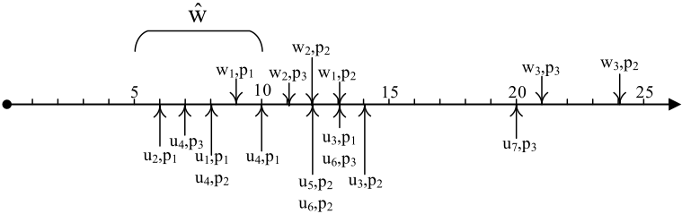
Example 2. Back to Example 1, Fig. 2 shows how to find the valid triple for w1 using Algorithm 1. In the window ̂ W, a valid triple (w1, p1, {u1, u2, u4}) is found by checking the covered pairs. The number of matched users reaches w1's capacity and the process of w1 terminates. Then, pairs related to u1, u2, u4 and p1 are removed while updating the timeline. After this, we construct new windows and repeat the above steps for w2 and w3. Valid triples of w2 and w3 are (w2, p2, {u3, u5, u6}) and (w3, p3, {u7}).
3.3 AlgorithmAnalysis
Complexity analysis. The complexity of building the timeline is O(|W| × |P | + |U| × |P |). The complexity of finding results for workers in ̂ W is O(δw × | ˜U|), where ˜U is the set of users in the covered pairs in ̂ W. Thus, the worst time complexity is O(|W| × |P | × |U| × |̂L|). The space complexity
Algorithm 1: Sliding Window
Input: W, U, P Output: M 1 Make a heap ∆ to store each w ∈ W ordered by their capacity 2 Construct a time line ̂L 3 while ∆ is not empty do 4 Pop w from∆ 5 Initialize an empty triple tri 6 Construct slide windoŵ W with length δw 7 while exists next ̂ W on ̂L do 8 Find a valid triple tri′ with the maximum number of users for (w, p) that is at the beginning of ̂ W 9 if |tri′ .Us| > |tri.Us| then 10 tri ← tri′ 11 if |tri.Us| == cw then 12 break 13 if tri is not empty then 14 Put tri intoM and update ̂L 15 returnM4 Threshold Scanning Algorithm
Recall that the Sliding Window greedily assigns users to workers ordered by their capacity. However, the number of users that a worker actually serves also depends on the locations and the departure time. Only focusing on capacity cannot achieve good results in many cases. To solve the problem more effectively, we further present a threshold-based algorithm, named Threshold Scanning.
4.1 Basic Idea
To improve the effectiveness, Threshold Scanning use a temporary storage. At the same time, we use a random threshold value to guarantee the efficiency. We divide the whole timeline into a set of intervals. In each interval, we greedily sort workers according to their capacity. Workers with a large capacity are matched preferentially. We randomly select a threshold value θ ∈ [1, cmax] based on the capacity of workers. For a triple (w, p,Us), if |Us| ≥ θ, it is the matching result of w and users in Us. If not, it is temporarily stored. These triples will be replaced if we can find a triple that can match more users.
4.2 AlgorithmDescription
We initialize the result set M, the temporary storage Cache and randomly choose a threshold θ ∈ [1, cmax] (Lines 1-2). Then, the timeline is divided into a set of intervals (Lines 3-4). In each interval Ii, all the pairs of workers are sorted in a heap ∆ and are popped one by one (Lines 5-7). If w and p have not been processed before and |tri.Us| ≥ θ, tri is put into M as a matching result (Lines 8-11). If |tri.Us| < θ, tri is stored into Cache (Lines 12-13). If w or p has been processed, we remove the triples related to w and p from Cache and find a new triple (Lines 14-16). If |tri.Us| meets the threshold, tri will be put intoM (Lines 17-18). If |tri.Us| is less than θ but larger than the triples that are removed before, tri is put into Cache (Lines 19-20). If there is no a better triple, we recover Cache (Lines 21-22). When the first scan finishes, triples in M and Cache are merged. In the second scan, we repeat the above steps with θ = 1 (Line 25).
Example 3. Back to Example 2. Suppose θ = 2 and we divide the whole timeline into 5 time intervals, each time
Algorithm 2: Threshold Scanning Input: W, U, P Output: M 1 M = ∅, Cache = ∅ 2 θ = randomly choosing an integer from {1, · · · , cmax} 3 Construct a time line ̂L 4 Divide ̂L into a set of intervals I 5 foreach Ii ∈ I do 6 Store (w, p) into ∆ ordered by the capacity of w 7 foreach (w, p) ∈ ∆ do 8 if w /∈ Cache and p /∈ Cache then 9 Find a valid triple tri for (w, p) with the maximum number of users 10 if |tri.Us| ≥ θ then 11 M = M ∪ {tri} 12 else 13 Cache = Cache ∪ {tri} 14 else if w ∈ Cache or p ∈ Cache then 15 Remove the triple related to w and p from Cache 16 Find a valid triple tri for (w, p) with the maximum number of users 17 if |tri.Us| ≥ θ then 18 M = M ∪ {tri} 19 else if |tri.Us| is larger than the realted triple in Cache then 20 Cache = Cache ∪ {tri} 21 else 22 Recovery Cache 23 24 M = M ∪ Cache, Cache = ∅ 25 Repeat Lines 5-23 with θ = 1 26 returnMinterval is 5 minutes. We skip I1, because it is empty. In I2, there is only one worker, the matching result of w1 is (w1, p1, {u1, u2, u4}) which the number of users is larger than θ. In I3, ∆ = {(w2, p3), (w2, p2)}. The matching result of (w2, p3) is (w2, p3, {u6}) and it is stored in Cache. The matching result of (w2, p2) is (w2, p2, {u3, u5, u6}) which meets the threshold. (w2, p3, {u6}) is removed from Cache. In I5, the matching result of (w3, p3) is (w3, p3, {u7}). It is stored in Cache. As all the workers are matched, the algorithm terminates. The final results are (w1, p1, {u1, u2, u4}), (w2, p2, {u3, u5, u6}) and (w3, p3, {u7}).
4.3 AlgorithmAnalysis
Complexity analysis. The complexity of building the timeline is O(|W| × |P | + |U| × |P |). The complexity of finding valid triples in a time interval is O(|∆| × | ˜U| × δw), where |∆| is the size of pairs stored in each interval. The worst time complexity is O(|W|×|P |×|U|×|̂L|). The space complexity is O(|W | × |P | + |U | × |P | + | ̂L|).
| Data | |W| | |P | | |U| | Capacity | Waiting Time |
|---|---|---|---|---|---|
| A B | 5 857 | 6 1027 | 20 4578 | [1,10] | [3,10] |
| C | 6247 | 5987 | 34972 |
| Factor | Setting |
|---|---|
| |W | |P | |U | σl of locations (Normal Distribution) σt of arriving time (Normal Distribution) θ | 2000, 4000, 6000, 10000, 20000 2000, 4000, 6000, 10000, 20000 10000, 20000, 30000, 50000, 100000 120, 140, 160, 180, 200 60, 70, 80, 90, 100 1, 4, 10 |
5 Experiment
In this section, we report the experimental results and corresponding analyses. We use both real and synthetic datasets in our experiments to verify the effectiveness, efficiency and scalability of our algorithms.
5.1 Experiment Setup
We conduct our algorithms over gMission [Chen et al., 2014]. In the dataset, each user who posts a task and each worker has a location, a departure time, a radius and a speed. Each workplace has a location. We generate the capacity of workers from 1 to 10, and the maximum waiting time is from 3 to 10 minutes. We extract 3 datasets according to the size of the regions. We also generate a synthetic dataset to test the algorithms. We generate the location and departure time of users, workers and workplaces following the uniform distribution. All users, workers and workplaces are located in a coordinate system of 800×800. The departure time is in 5 hours. To verify the impact of data distribution, we also generate another dataset following the normal distribution. In the datasets, the capacity of each worker varies from 1 to 10. The waiting time of workers varies from 5 to 10 minutes, and the waiting time of users varies from 1 to 5 minutes. The maximum radius of workers as 80, and the maximum radius of users as 40. We set the travel speed of workers is 8 and the travel speed of users is 4. The details of real and synthetic datasets are illustrated in Table 2 and 3 and the default settings are bold.
Compared algorithms. We evaluate our Sliding Window algorithm (shorted as "WIN") and Threshold Scanning algorithm (shorted as "TS") with approaches in [Li et al., 2019], MWIS, GSM, DSM and PATH. We add the temporal constrain in MWIS while constructing the graph such that it still can find the optimal solution in SAM. We remove the invalid triples from the matching results of GSM, DSM and PATH. We execute the algorithms 10 times and report the average results. To further analyze the impact of θ of TS, we select three different θ in the synthetic datasets (shorted as "TS-1", "TS-4" and "TS-10"). We evaluate the effectiveness of the algorithms using the metric of the matching size. We evaluate the efficiency of the algorithms by reporting the running time and memory cost. We conduct the experiments in a machine with Intel Xeon Silver 4110 and 512GB main memory.
With the increase of |W|, |P| and |U|, we can observe that the matching size of all the algorithms increases. When |W| gets larger, the matching size of WIN becomes much smaller than TS-4. The reason is that TS can retain those workers who match more users by adjusting the triples so that it can match more users when the number of workplace is much smaller than the number of workers. When |P| = 20000, the matching size of WIN is larger than TS-4. The reason is that workers have more alternative workplaces to serve users, and workers are likely to match more users. Similarly, the increase of |U| also improves the number of users that each worker could match.
Matching size w.r.t σ. Fig. 4(j) and 4(m) report the results of matching size w.r.t σ of locations and arriving time. We can observe that the matching size decreases with the increase of σl and σt. When σl increases, the locations become decentralized. The number of workplaces that workers and users can reach decreases gradually, leading to the decrease of matching size. When σt increases, the number of workplaces that workers and users can reach stays the same, but the arriving time gets decentralized. Some valid triples will be removed since they does not satisfy the temporal constraint. We also observe that WIN could get a better result than TS-4 if the distribution is centralized enough.
Running time w.r.t θ. According to the results in the second column of Fig. 4, TS-1 runs the fastest. The reason is that it stores all the valid triples without other operations. The running time of TS increases with the increase of θ. When θ equals to 10, TS-10 costs more time than WIN and TS-4. The reason is that most triples are stored in the cache, and TS-10 has to constantly search whether there are better triples. The running time of TS-4 is similar to WIN.
Running time w.r.t |W|, |P| and |U|. Fig. 4(b), 4(e) and 4(h) show the results of running time w.r.t |W|, |P| and |U|. With the increase of |W|, |P| and |U|, all the algorithms cost more time to find the solution. GSM, DSM and PATH run much faster. The reason is that they only consider the stable constrain and ignore the temporal constraint.
Running time w.r.t σ. Fig. 4(k) and 4(n) report the results of running time w.r.t σ of locations and arriving time. The increase of σl and σt has opposite effects on running time. With the increase of σl, all the algorithms run faster. The
5.2 Results on Real Datasets
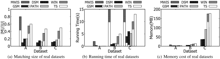
In this section, the experiments are conducted over the real datasets of gMission and we verify the effectiveness and efficiency of the algorithms, shown in Fig. 3.
Effectiveness w.r.t matching size. From Fig. 3(a), MWIS can output a best matching result in dataset A, but it cannot output the result within an acceptable time in larger datasets because the complexity is too high. GSM is the worst of all the cases. The performance of PATH and DSM is a bit better than GSM in the datasets. The matching size of TS and WIN are larger than GSM, DSM and PATH. The matching size of TS is larger than WIN. TS improves the effectiveness by 5%-15%. This means that our algorithms are better than the existing approaches which verifies the effectiveness.
Efficiency w.r.t time and memory cost. The running time and memory cost are shown in Fig. 3(b) and 3(c). The running time of MWIS is longer than the others and it cannot out put a result in dataset B and C before we terminate it. WIN runs faster than TS. The running time of GSM is less than other algorithms and PATH is a little more efficient than DSM. The memory cost of MWIS is the largest in dataset A. Due to it does not output a result, we do not record its memory in dataset B and C. Except MWIS, the memory cost by TS and WIN is the largest in dataset B and C. The memory cost of GSM and DSM is similar in all the datasets. The memory cost of PATH is larger than GSM and DSM.
5.3 Results on Synthetic Dataset
We test the scalability by comparing the algorithms on the synthetic datasets. The results are shown in Fig. 4.
Matching size w.r.t θ. According to the results in the first column of Fig. 4, we can observe that the matching size of TS gets larger as θ increases. The matching size of TS-4 and TS-10 are larger than WIN at most cases. TS-10 improves the effectiveness by about 10%-20%. The matching size of TS1 is the smallest because a triple will be saved if the worker can match at least one user regardless of whether there is a better triple. It leads to a waste of the capacity. With the increase of θ, TS replace these triples by better results.
Matching size w.r.t |W|, |P| and |U|. Fig. 4(a), 4(d) and 4(g) report the results of matching size w.r.t |W|, |P| and |U|.
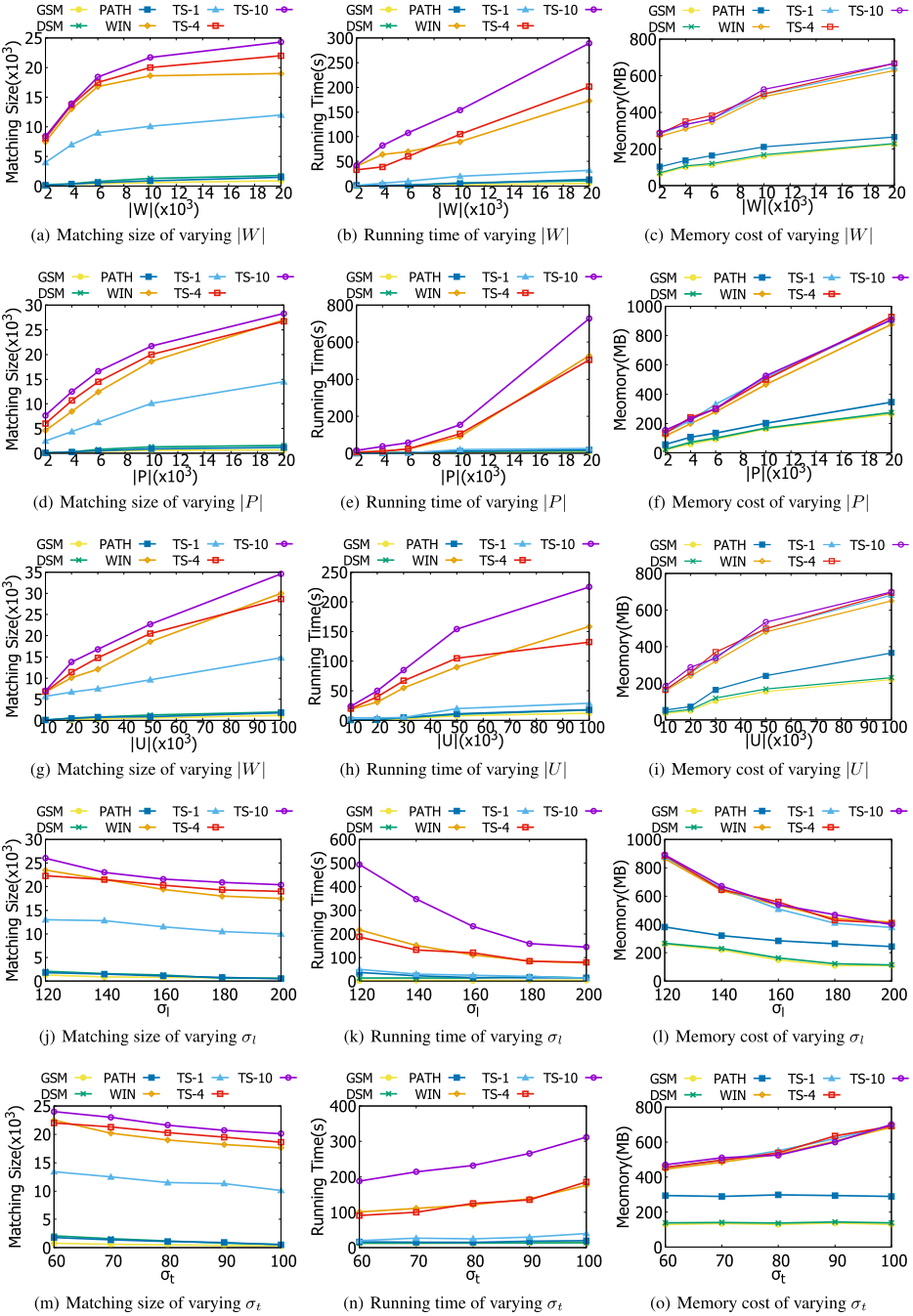
reason is that the number of workplaces that each worker and user can reach decreases, the time of enumerating triples goes down. On the contrary, the running time increases with the increase of σt. The reason is that the timeline gets longer when the arriving time is more decentralized. It costs more time to find triples in the timeline. The changing of σt does not affect the running time of GSM, DSM and PATH as they do not consider the temporal constrain.
Memory cost w.r.t θ. According to the results in the last column of Fig. 4, the memory cost of TS and WIN are similar. The change of θ has a slight impact on memory cost.
Memory cost w.r.t |W|, |P| and |U|. Fig. 4(c), 4(f) and 4(i) show the memory cost of running time w.r.t |W|, |P | and |U|. With the increase of |W|, |P| and |U|, the memory cost of all the algorithms increase. The memory cost of TS and WIN increase rapidly, because they need to build the timeline which cost much memory. GSM and DSM only store the basic information, therefore the memory cost of them are similar and are less than others. PATH needs to build the index, therefore it costs more memory than GSM and DSM.
Memory cost w.r.t σ. Fig. 4(l) and 4(o) report the results of memory cost w.r.t σ of locations and arriving time. The distributions of locations and arriving time still show opposite effects. The memory cost decreases with the increase of σl. On the one hand, the decrease of matching size saves some memory. On the other hand, the number of pairs of the timeline decreases a lot which is the main reason. When σt increases, the timeline gets longer, TS and WIN need cost more memory to store the timeline. The changing of σt still does not affect the memory of GSM, DSM and PATH.
6 RelatedWork
In this section, we review related work in spatial crowdsourcing from three categories, offline task assignment, online task assignment and preference-aware task assignment.
Offline task assignment. In the offline scenario, studies [Kazemi and Shahabi, 2012][To et al., 2015][Gao et al., 2016] know the global spatial and temporal information. Xia et al. [Xia et al., 2019] formulated a PTA problem which aimed to maximize the profit of the spatial crowdsourcing platform. Tong et al. [Tong et al., 2018b] gave a unified formulation of ride sharing problem and proposed insertionbased algorithms to solve it. Studies of EBSN [Cheng et al., 2017b][She et al., 2017][She et al., 2015] focused on how to make plans to participate in events.
Online task assignment. In the online scenario, workers and users dynamically appear on the platform, the global spatial and temporal information cannot be known in advance. Competitive ratio [Karp et al., 1990] is usually used to evaluate the performance of the algorithms. Tong et al. [Tong et al., 2016] analyzed the performance of existing algorithms through experimental results. Tong et al. [Tong et al., 2017] tried to predict the taxi demand and guided the drivers based on the result of prediction methods. With the rise of new spatial crowdsourcing platforms, Song et al. [Song et al., 2017] proposed a 3D matching as a consequence, calculating the online matching. The aforementioned studies have achieved good results in 2D and 3D problems. However, they fail to consider the services preference of users and workers. Thus, the algorithms cannot be applied to our problem.
Preference-aware matching. The individual preference is an important factor to improve the satisfaction of the assignment. Stable marriage [Gale and Shapley, 2013] is a typical matching problem which considers the preference between men and women. In recent studies, researchers combine the individual preference with the spatial and temporal information. Zhao et al. [Zhao et al., 2019a] proposed two matching approaches to find a stable assignment in the taxi-calling platform. The preferences between users and drives were distance and profit. Zhao et al. [Zhao et al., 2019b] presented a method to learn the preference in historical data and used three approaches to get a task assignment. These studies only focused on 2D matching problem, which cannot be extended to our problem. Li et al. [Li et al., 2019] proposed a 3D stable matching. In that matching result, for each pair of match worker and user, there is no place that is closer to both the matched worker and user. They can make sure that no matched workers and users both prefer a second workplace to the matched one. Unfortunately, it ignored an important factor that the workers and users matched to the same workplace should arrive almost at the same time. Thus, the algorithms cannot achieve a good result in SAM.
7 Conclusion
In this paper, we propose a new stable matching problem called the Simultaneous Arrival Matching (SAM). We prove that the SAM is NP-hard and the monotonic additivity of the matching results. To solve the problem effectively and efficiently, we devise Sliding Window and Threshold Scanning. We compare our algorithms with existing approaches and the experimental results show the effectiveness and efficiency. In summary, Threshold Scanning could achieve a better result than Sliding Window at most cases. Threshold Scanning can solve the problem effectively and efficiently when a suitable threshold is selected. As for the future work, we will study distributed and parallel algorithms in larger realworld datasets, and explore the preference between workers and users to improve the satisfaction.
Acknowledgements
Yurong Cheng is supposed by the NSFC (Grant No. 61902023, U1811262). Ye Yuan is supported by the NSFC (Grant No. 61932004, 61572119 and 61622202) and the Fundamental Research Funds for the Central Universities (Grant No. N181605012). Guoren Wang is supported by the NSFC (Grant No. 61672145 and 61732003). Lei Chen's work is partially supported by the Hong Kong RGC GRF Project 16207617, CRF Project C6030-18GF, AOE Project AoE/E603/18, China NSFC No. 61729201, Guangdong Basic and Applied Basic Research Foundation 2019B151530001, Hong Kong ITC ITF grants ITS/044/18FX and ITS/470/18FX, Didi-HKUST joint research lab project, Microsoft Research Asia Collaborative Research Grant and Wechat and Webank Research Grant. Guoren Wang is the corresponding author of this work.
@inproceedings{ijcai2020p178,
  title     = {Simultaneous Arrival Matching for New Spatial Crowdsourcing Platforms},
  author    = {Li, Boyang and Cheng, Yurong and Yuan, Ye and Wang, Guoren and Chen, Lei},
  booktitle = {Proceedings of the Twenty-Ninth International Joint Conference on
               Artificial Intelligence, {IJCAI-20}},
  publisher = {International Joint Conferences on Artificial Intelligence Organization},
  editor    = {Christian Bessiere},
  pages     = {1279--1287},
  year      = {2020},
  month     = {7},
  note      = {Main track},
  doi       = {10.24963/ijcai.2020/178},
  url       = {https://doi.org/10.24963/ijcai.2020/178},
}
TY - CPAPER TI - Simultaneous Arrival Matching for New Spatial Crowdsourcing Platforms AU - Li, Boyang AU - Cheng, Yurong AU - Yuan, Ye AU - Wang, Guoren AU - Chen, Lei T2 - Proceedings of the Twenty-Ninth International Joint Conference on Artificial Intelligence, IJCAI-20 PB - International Joint Conferences on Artificial Intelligence Organization PY - 2020 SP - 1279 EP - 1287 DO - 10.24963/ijcai.2020/178 UR - https://doi.org/10.24963/ijcai.2020/178 ER -Copied
Machine-readable versions of this paper, for tools and AI agents:





