
Cause-Effect Association between Event Pairs in Event Datasets
Proceedings of the Twenty-Ninth International Joint Conference on Artificial Intelligence. Main track. Pages 1202-1208.
https://doi.org/10.24963/ijcai.2020/167
Keywords
- Machine Learning: Time-series;Data Streams
- Knowledge Representation and Reasoning: Action, Change and Causality
- Data Mining: Mining Spatial, Temporal Data
Abstract
Causal discovery from observational data has been intensely studied across fields of study. In this paper, we consider datasets involving irregular occurrences of various types of events over the timeline. We propose a suite of scores and related algorithms for estimating the cause-effect association between pairs of events from such large event datasets. In particular, we introduce a general framework and the use of conditional intensity rates to characterize pairwise associations between events. Discovering such potential causal relationships is critical in several domains, including health, politics and financial analysis. We conduct an experimental investigation with synthetic data and two real-world event datasets, where we evaluate and compare our proposed scores using assessments from human raters as ground truth. For a political event dataset involving interaction between actors, we show how performance could be enhanced by enforcing additional knowledge pertaining to actor identities.
- [Acharya, 2014] S. Acharya. Causal Modeling and Prediction over Event Streams. PhD thesis, University of Vermont, 2014.
- [Ale and Rossi, 2000] J.M. Ale and G.H. Rossi. An approach to discovering temporal association rules. In Proc. of the ACM Sym- posium on Applied Computing, pages 294-300, 2000.
- [Allan, 2002] J. Allan, editor. Topic Detection and Tracking: Event- based Information Organization. Kluwer Academic Publishers, Norwell, MA, USA, 2002.
- [Baeza-Yates and Ribeiro-Neto, 2011] R. Baeza-Yates and B. Ribeiro-Neto. Modern Information Retrieval. New York: ACM Press;
- [Bhattacharjya et al., 2018] D. Bhattacharjya, D. Subramanian, and T. Gao. Proximal graphical event models. In Proc. of NeurIPS, pages 8147-8156, 2018.
- [Bhattacharjya et al., 2020] D. Bhattacharjya, K. Shanmugam, T. Gao, N. Mattei, K. R. Varshney, and D. Subramanian. Event- driven continuous time Bayesian networks. In Proc. of the 34th AAAI, 2020.
- [Chambers and Jurafsky, 2008] N. Chambers and D. Jurafsky. Un- supervised learning of narrative event chains. In Proc. of the ACL, volume 94305, pages 789-797, 2008.
- [Church and Hank, 1990] K. W. Church and P. Hank. Word asso- ciation norms, mutual information, and lexicography. Computa- tional Linguistics, 16(1):22-29, 1990.
- [Cooper, 1997] G. F. Cooper. A simple constraint-based algorithm for efficiently mining observational databases for causal relation- ships. Data Mining and Knowledge Discovery, 1(2):203-224, 1997.
- [Cox and Lewis, 1972] D. R. Cox and P. A. W. Lewis. Multivari- ate point processes. In Proc. of the 6th Berkeley Symposium on Mathematical Statistics and Probability, Volume 3: Probability Theory, pages 401-448, 1972.
- [Cox, 1992] D. R. Cox. Causality: Some statistical aspects. Journal of the Royal Statistical Society, Ser. A, 155:291-301, 1992.
- [Didelez, 2008] V. Didelez. Graphical models for marked point processes based on local independence. Journal of the Royal Sta- tistical Society, Ser. B, 70(1):245-264, 2008.
- [Eels, 1991] E. Eels. Probabilistic Causality. Cambridge Univer- sity Press, 1991.
- [Frank and Asuncion, 2010] A. Frank and A. Asuncion. UCI ma- chine learning repository, 2010.
- [Granger, 1969] C. W. J. Granger. Investigating causal relations by econometric models and cross-spectral methods. Econometrica, 37:424-438, 1969.
- [Gunawardana and Meek, 2016] A. Gunawardana and C. Meek. Universal models of multivariate temporal point processes. In Proc. of the 19th AISTATS, pages 556-563, 2016.
- [Gunawardana et al., 2011] A. Gunawardana, C. Meek, and P. Xu. A model for temporal dependencies in event streams. In Proc. of NeurIPS, pages 1962-1970, 2011.
- [Khan and Soutchanski, 2018] S. M Khan and M. Soutchanski. Di- agnosis as computing causal chains from event traces. In Proc. of the AAAI Fall Symposium on Integrating Planning, Diagnosis, and Causal Reasoning, 2018.
- [Kleinberg and Mishra, 2009] S. Kleinberg and B. Mishra. The temporal logic of causal structures. In Proc. of the 25th UAI, pages 303-312, 2009.
- [Leetaru and Schrodt, 2013] K. Leetaru and P. A. Schrodt. GDELT: Global data on events, location, and tone. In International Studies Association (ISA) Annual Convention, 2013.
- [Li and Ma, 2004] T. Li and S. Ma. Mining temporal patterns with- out predefined time windows. In Proc. of the ICDM, pages 451- 454, 2004.
- [Luo et al., 2016] Z. Luo, Y. Sha, K. Q. Zhu, S. Hwang, and Z. Wang. Commonsense causal reasoning between short texts. In Proc. of the 15th KR, pages 421-430, 2016.
- [Mannila et al., 1997] H. Mannila, H. Toivonen, and A. I. Verkamo. Discovery of frequent episodes in event sequences. Data Mining and Knowledge Discovery, 1:259-289, 1997.
- [Meek, 2014] C. Meek. Toward learning graphical and causal pro- cess models. In Proc. of the UAI Workshop on Causal Inference: Learning and Prediction, pages 43-48, 2014.
- [O'Brien, 2010] S. P. O'Brien. Crisis early warning and decision support: Contemporary approaches and thoughts on future re- search. International Studies Review, 12:87-104, 2010.
- [Okada et al., 2015] Y. Okada, K. I. Fukui, K. Moriyama, and M. Numao. Causal inference with time and space proximity un- der uncertainty. In Pacific-Asia Conference on Knowledge Dis- covery and Data Mining, pages 293-304, 2015.
- [Pearl, 2009] J. Pearl. Causality: Models, Reasoning and Inference. Cambridge University Press, New York, NY, USA, 2nd edition, 2009.
- [Pearl, 2014] J. Pearl. Probabilistic Reasoning in Intelligent Sys- tems: Networks of Plausible Inference. Morgan Kaufmann, 2014.
- [Radinsky et al., 2012] K. Radinsky, S. Davidovich, and S. Markovitch. Learning to predict from textual data. Journal of Artificial Intelligence Research, 45:641-684, 2012.
- [Rajaram et al., 2005] S. Rajaram, T. Graepel, and R. Herbrich. Poisson-networks: A model for structured point processes. In Proc. of the 10th AISTATS, pages 277-284, 2005.
- [Riaz and Girju, 2010] M. Riaz and R. Girju. Another look at causality: Discovering scenario-specific contingency relation- ships with no supervision. In Proc. of the 4th IEEE Int. Conf. on Semantic Computing (ICSC), pages 361-368, 2010.
- [Silverstein et al., 2000] C. Silverstein, S. Brin, R. Motwani, and J. Ullman. Scalable techniques for mining causal structures. Data Mining and Knowledge Discovery, 4(2-3):163-192, 2000.
- [Simma and Jordan, 2010] A. Simma and M. I. Jordan. Modeling events with cascades of Poisson processes. In Proc. of the 26th UAI, pages 546-555, 2010.
- [Singh et al., 2002] P. Singh, T. Lin, E. T. Mueller, G. Lim, T. Perkins, and W. L. Zhu. Open mind common sense: Knowledge acquisition from the general public. In On the Move to Meaningful Internet Systems 2002: CoopIS, DOA, and ODBASE), pages 1223-1237, 2002.
- [Sohrabi et al., 2017] S. Sohrabi, A. V. Riabov, and O. Udrea. State projection via AI planning. In Proc. of the 31st AAAI, 2017.
- [Spirtes et al., 2001] P. Spirtes, C. Glymour, and R. Scheines. Causality, Prediction, and Search. MIT Press, Cambridge, MA, USA, 2nd edition, 2001.
- [Suppes, 1970] Patrick Suppes. A Probabilistic Theory of Causal- ity. Amsterdam: North-Holland Publishing Company, 1970.
- [Weiss and Page, 2013] J. C. Weiss and D. Page. Forest-based point process for event prediction from electronic health records. In Machine Learning and Knowledge Discovery in Databases, pages 547-562, 2013.
References were extracted automatically from the PDF and may contain errors.
Full text extracted automatically from the PDF; figures, tables and equations may differ. The PDF is the version of record.
1 Introduction
Discovering causal relationships from observational data is widely studied in AI and remains of fundamental interest in scientific endeavors [Cox, 1992; Spirtes et al., 2001; Pearl, 2009]. In this paper, we study causal association between pairs of events, where an event is defined abstractly as "a particular thing that happens at a specific time and place, along with all necessary preconditions and unavoidable consequences" [Allan, 2002]. We assume access to an event dataset, i.e. data about occurrences of various types of events over the timeline. Event datasets are different from time series data in that they typically entail arrivals at irregular epochs (such as medical events), rather than continuousvalued measurements at regular epochs (such as daily stock prices). Large event datasets are increasingly common in domains such as maintenance, health, politics and finance.
Our objective is to build a computational system that identifies potential causal associations from large event datasets. Such a system could provide data-driven support to analysts, assisting them with thoughtful and reasoned analysis about potential future states of the world. Recent efforts to design systems that discover and use pairwise causal associations for downstream reasoning and processing include work by Radinsky et al. [2012], who identify cause-effect pairs from news articles and make predictions about potential future events by generalizing the causal relationships. Luo et al. [2016] also learn cause-effect pairs from text, representing these relationships in a graph. Sohrabi et al. [2017] describe a scenario generation system based on a planning formulation; as input, they use expert-provided 'mind maps' that capture causal connections among concepts. Pairwise causal knowledge has also been assessed through crowd sourcing, such as in the open mind common sense project [Singh et al., 2002].
Existing systems for identifying cause-effect relations rely on unstructured text or human-assessed representations, joint independent and identically distributed (i.i.d.) observations of random variables without temporal information, or traditional time series data (over regular epochs) as in Granger causality [Granger, 1969]; in contrast, we investigate learning causal associations using structured event datasets as input. This complements existing related research as it provides another route for causal discovery from real-world data, with numerous downstream applications. Note that we restrict our attention to association between pairs of events as opposed to more complex structures, for the practical reason that it is significantly easier for users/analysts to understand pairwise associations rather than conditional causal relationships. Furthermore, it is crucial for our methods to be scalable in both the number of types of events as well as the size of the dataset.
Contributions. We propose a suite of algorithms that generate scores for causal relationships between pairs of events in structured datasets. We introduce a novel framework that incorporates all the scores and propose a continuous-time point process approach that uses the ratio of conditional intensity rate parameters from a graphical representation. We analyze the complexity and correctness of our scores theoretically as well as compare them in experiments involving synthetic and two real-world datasets: 1) a diabetes dataset [Frank and Asuncion, 2010; Acharya, 2014], and 2) the ICEWS political event dataset [O'Brien, 2010] - a relational (dyadic) event dataset where events are interactions between two actors. Our scores outperform baselines from the literature.
2 RelatedWork
Event Models. There has been substantial work around studying event datasets, spanning several analytical domains.
In statistics, there is a long history of modeling such datasets as multivariate point processes [Cox and Lewis, 1972]. In data mining, event datasets have been used for identifying patterns and making predictions [Mannila et al., 1997]. The literature has spilled over into AI and machine learning, yielding sophisticated temporal processes including Poisson nets [Rajaram et al., 2005], Poisson cascades [Simma and Jordan, 2010], piecewise-constant conditional intensity models [Gunawardana et al., 2011], forest-based point processes [Weiss and Page, 2013], proximal graphical event models [Bhattacharjya et al., 2018], and event-driven continuous time Bayesian networks [Bhattacharjya et al., 2020].
Didelez [2008] and Gunawardana and Meek [2016] proposed graphical event models (GEMs) as a framework to generalize many of the afore-mentioned multivariate temporal processes. They can be viewed through a causal lens, much like causal networks can be seen as directed graphical models [Pearl, 2014] imbued with causal semantics. Although GEMs are theoretically broad in scope, specific assumptions about historical dependencies are required to learn models in practice. Furthermore, an edge in a GEM from event y to x does not necessarily correspond to a causal association as defined in this paper. Our work is the first to propose pairwise scores using conditional intensity rates that are based on the multivariate point process framework behind GEMs.
Causal Association in NLP. Most of the work on pairwise causal associations appears in natural language processing and computational linguistics, where events are often merely textual phrases. Much of this literature revolves around the fundamental idea that 'causes' change the probabilities of their 'effects' [Suppes, 1970]. For a pair of events (y, x), y could potentially be a cause of effect x if x happens more frequently when y happens relative to its base rate, i.e. p(x|y) > p(x). Although this approach identifies dependence between events, there are clearly caveats towards its usage for discovering causal relationships. For instance, (y, x) could have a common cause z and still satisfy p(x|y) > p(x).
Despite its limitations, pairwise co-occurrence has been popular in causal discovery from text since Church and Hank [1990] proposed the use of mutual information for word association, computed by identifying co-occurrence of words in a corpus. Riaz and Girju [2010] and Luo et al. [2016] deploy discourse cues (such as 'if A then B') together with statistical co-occurrence based scores for discovering causeeffect pairs in text. In the following section, we extend these scores to account for temporal order event datasets.
Other Causal Association. We briefly mention a select few other domains in which causal association has been explored. These include unsupervised data mining approaches such as association rule mining [Cooper, 1997; Silverstein et al., 2000; Ale and Rossi, 2000], clustering [Okada et al., 2015] and temporal pattern mining [Li and Ma, 2004], as well as using logical formulations [Kleinberg and Mishra, 2009] and planning and situational calculus for causal event detection [Khan and Soutchanski, 2018], etc. Our work is closer in spirit to event models and pairwise association in NLP.
3 Cause-Effect Association Scores
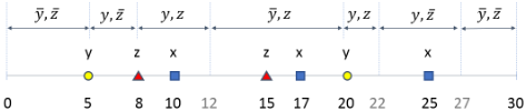
An event dataset is a sequence of events, D = {Di}Ni=1 . Each event Di is a tuple (xi, ti) where xi is the event label/type and ti is the time of occurrence, ti ∈ R+. We assume a strictly temporally ordered dataset, ti < tj for i < j, initial time t0 = 0 and end time tN+1 = T . y, x refer to an arbitrary pair of event types belonging to label set L whose cardinality is M, i.e. |L| = M. Figure 1 depicts an example event dataset with N = 7 events across M = 3 event labels over a horizon of T = 30 days (a month).
In this section, we begin by proposing a general framework for computing causal association scores from an event dataset. To illustrate the generality and practicability of this framework, we first extend the scores from computational linguistics; these are purely data-driven and based only on temporal co-occurrence. We then propose scores based on generative models with conditional intensity rates of events.
3.1 AGeneral Framework
A popular approach to causal modeling is based on independence tests [Pearl, 2009]. However, high-dimensional tests can be intractable in general causal relationships. To discover causal event pairs, we adopt the same paradigm and consider the following framework of hypothesis testing:
where (y, x) is the pair to be tested such that y occurs before x, and z is a joint random variable indicating whether event labels in the set Z ⊆ L have occurred or not. The null hypothesis tests if P(x|y, z) and P(x|z) are from the same distribution, which indicates y has no impact on x, conditioned on some other variables Z, and hence cannot be a cause for x [Pearl, 2014]. In this work, a cause-effect association entails that y makes x more likely in the future. The probabilities can be modeled with different methods and the independence tests can use different metrics, but the general form to be evaluated is f(P(x|y, z), P(x|z)).
Note that as defined above, where y and z occur before x, P(x|y, z) > P(x|z) implies that P(y|x, z) > P(y|z). This 'backwards' view is promoted in NLP in particular. In the remainder of this section, we propose specific scores and briefly mention their connection to the general framework.
3.2 Temporal Co-occurrence Based Scores
We first investigate some baseline scores inspired by related temporal co-occurrence association work [Church and Hank, 1990], with scores like p(y|x) and p(x|y) .
To make the computation of p(y|x) and p(x|y) in event datasets tractable, where there could be multiple occurrences of y and x that are staggered over T , we take a window-based view of co-occurrence, making the assumption that causal influence is prevalent only for a limited time after an event occurs. For time window w, we compute these two conditional probabilities as:
where p(y) and p(x) are the probabilities of observing events y and x respectively, i.e. p(y) = N(y)/T and p(x) = N(x)/T for event counts N(y) and N(x) over the horizon T . pw (y � x) is computed from the event dataset by counting occurrences of data where x occurs and at least one y event occurs within the preceding time window (between times 0 and T), pw (y � x) = N w (y � x)/T. p(y � x) is computed by counting the number of occurrences where y occurs and at least one x event occurs within a feasible forward time window of length w, pw (y � x) = N w (y � x)/T. Every pair (y, x) is associated with support computed as sw (y, x) = min {N w (y � x), N w (y � x)}.
Using the two conditional probabilities, we propose novel adaptations of cause-effect scores from causal discovery work in text: necessity sufficiency trade-off (NSTE) score from Luo et al. [2016] (the subscript signifies adaptation to an event dataset) and event control dependency (ECDE) score from Riaz and Girju [2010]. NSTE requires a base rate penalization parameter α ≥ 0 and a parameter λ ∈ [0, 1] that trades off necessity (first term) and sufficiency (second term) scores as follows:
Both necessity and sufficiency terms involve a penalization in the denominator using the parameter α which prevents frequent events from being considered as highly causally associative merely on the basis of chance; higher values result in more penalization for frequent events.
Remark 1. NSTE follows the General Framework (1) by assuming Z = ∅ and using a test statistic that is a weighted geometric mean of the 'forward' ratio pw (x|y) p(x)α (sufficiency) and the 'backward' ratio pw (y|x) p(y)α (necessity).
ECDE score, on the other hand, maximizes over two terms that are essentially proxies for necessity and sufficiency causality, ECDE(y, x) = max {TN , TS}, where:
and sufficiency term TS is similar, with arrows in the other direction and p(y) replacing p(x) in the first term. γ ≥ 0 is a parameter to prevent a zero denominator and can be set to a low number (such as 0.01). TN is a product of an adjusted odds term for y|x and a term that captures the importance of the effect x as compared to all other potential effects v.
Remark 2. ECDE follows the General Framework (1) by assuming Z = ∅ and using a test statistic that maximizes over 'forward' (sufficiency) and 'backward' (necessity) components. The backward component multiplies the odds of y|x with a factor that depends on other effects and is highest when x is the effect with maximum pw (y � x). The forward component is analogous.
The ECDE score is different from NSTE in that it also considers all other potential effects of cause y. It also uses normalization twice in computing ratios. The following theorem provides time complexity results for both these scores. Recall that N and M refer to the number of events and event labels respectively.
Theorem 1. The worst case time complexities for obtaining pairwise causal association scores for all event label pairs in L using NSTE and ECDE are O(MN +M 2 ) and O(MN +M 3 ) respectively.
Limitation. The above adapted scores suffer from a few shortcomings. p(x) and p(y) are interpretable as probabilities only in the special case where we have a finite set of time periods and where there is at most one event occurrence per event label in each time period. When events may appear irregularly on the timeline, these definitions are not probabilities. One can see that p(x) and p(y) represent gross (average) arrival rates that have dimensions of count per unit time, unlike probability which is dimensionless, and they are therefore sensitive to the units in which time is measured. This renders the above extension ad-hoc in general, even though it could be useful in practice. This motivates us to investigate scores that are applicable in a continuous-time setting, devoid of arbitrary parameters like α, λ or γ and more mathematically principled, as described next.
3.3 Conditional Intensity Based Scores
Event datasets can be modeled as marked point processes using conditional intensity functions λx(t|H) > 0 that represent the rate at which events of type x occur at time t given the history H [Didelez, 2008]. Since we are concerned with association between a pair (y, x), we begin by making a simplifying assumption: suppose the intensity of x at any time only depends on whether at least one event of type y has occurred in the preceding window w. Furthermore, for now, suppose that the rate at which x occurs does not depend on any other event label besides y. This entails that x has only two intensity parameters: λwx|y and its complement λwx|¯ y .
Making no other assumptions about the history dependent intensities of other event types (including y), it can be shown that the maximum likelihood estimates for both parameters for x can be computed using summary statistics:
where count N w (y � x) is as defined in the previous section and duration Dw (y) = ∑N+1 i=1 ∫ ti ti-1 I w y (τ)dτ is the duration over the entire time period from 0 to T for which condition y is true, given time window w. In the formal definition of Dw (y), I w y (t) is an indicator for whether y has occurred at least once in the feasible window w preceding time t. Note that the counts and durations for any number of event pairs can be computed in a single pass through the event dataset.
We introduce causal association scores that reflect how the conditional intensity of effect x is modified by the presence or absence of potential cause y. Specifically, we propose the following two conditional intensity ratios:
where the latter uses the complement (C) as a reference vs. the former which considers the base rate (B) λx = N(x)/T .
Remark 3. CIRB and CIRC follow the General Framework (1) by assuming p(x|y, z) = pdτ (x|y) = λwx|y dτ and p(x|z) = pdτ (x) = λxdτ . The test statistic for CIRB is the ratio of p(x|y, z) and p(x|z) whereas for CIRC it is the ratio of p(x|y, z) and p(x|¯ y, z).
Define CIRB\C as either CIRB or CIRC. We highlight a situation under which these scores are consistent.
Theorem 2. If at most only y's occurrences in a historical window w can impact the occurrence of x at any time s.t. λx|H(t) = λwx|y ∀t, where H(t) is the event history at time t, given sufficient data, CIRB\C = 1 indicates independence and CIRB\C ̸= 1 indicates dependence for the pair (y, x).
Proof. If in the underlying true relationship P(x|y, z) = P(x|z), then λwx|y dτ = λxdτ ⇒ λwx|y λx = 1, hence CIRB\C = 1 indicates independence. Else if P(x|y, z) ̸= P(x|z), then λwx|y λx ̸= 1 hence CIRB\C ̸= 1 indicates dependence. Conversely, if CIRB\C = 1, then λwx|y λx = 1 ⇒ λwx|y dτ = λxdτ ⇒ P(x|y, z) = P(x|z). Similarly, if CIRB\C ̸= 1, then (x|y, z) ̸= P(x|z).
In practice, the assumption that an effect x only depends on the history of potential cause y is likely unrealistic. A more general formulation allows x to depend on historical occurrences of any other event label; in the literature on graphical event models, this is captured by a (potentially cyclic) representation where the rate at which an event label occurs at any time depends only on the historical occurrences of its parents.
For a pair (y, x), suppose that x not only has y as a parent but also the set of labels Z. If x's rate depends on whether or not any of its parents y ∪ Z have occurred in the preceding window w, then there are 2|Z|+1 conditional intensity rates, maximum likelihood estimates of which can be determined through summary statistics, similar to equation (5):
where the counts and durations are generalizations of the previous definitions and can be computed similarly. Figure 1 illustrates how the timeline partitions various conditions for labels y and z, assuming window w = 7 days. In this example, D(¯ y, z) = D(y, ¯ z) = D(¯ y, ¯ z) = 8 days each and D(y, z) = 6 days. The maximum likelihood estimate for rate λwx|y,z = N w (y, z � x)/Dw (y, z) = 1/6.
Since we are interested in the pairwise association for (y, x), we suggest using the aggregate impact of y on x over all possible conditions of the other parental influences z. In this way, the score for the pair (y, x) measures how much y changes the rate at which x happens, averaged over all other potential parent states. Formally,
when y is a parent of x and otherwise the score is 0; the subscript M denotes that x could have multiple influences and g(·) is an aggregation of ratios over all z. We consider min. and max. aggregate functions as well as average (avg).
Note that the CIRM score can be viewed as a generalization of CIRC. Support for all CIR scores is assumed to be sw (y, x) = N w (y � x).
Remark 4. CIRM follows the General Framework (1) by assuming p(x|y, z) = pdτ (x|y, z) = λx|y,zdτ and p(x|z) = pdτ (x|z) = λx|zdτ . Moreover, the test statistic for CIRM is some aggregated ratio of p(x|y, z) and p(x|¯ y, z).
In order to discover the parents of x, we follow structure search like in other work on graphical event models [Meek, 2014; Bhattacharjya et al., 2018]. The log likelihood of the dataset for event label x with parents U is:
where u is an instantiation of parents U. In our experiments, we first learn the parent set of x that maximizes the BIC score by searching for any additional parents Z (other than y) through a forward-backward search - a standard approach in structure learning in graphical models - and then compute the CIRM score using the relevant summary statistics computed on the (optimal) learned graph, see equation (7). The BIC score is the sum of the log likelihood and a penalty term that incorporates the complexity of the model, determined by the total number of parents (Z+1) and equals 2|Z|+1 log(T); it is known to be asymptotically consistent for graphical event models [Meek, 2014].
Theorem 3. The worst case time complexity for obtaining pairwise causal association scores for all event label pairs in L using either CIRB or CIRC is O(MN +M 2 ). For CIRM, assuming that event labels occur in similar proportions in the event dataset, it is O(M 3N).
Proof. Using the same argument as in the proof of Theorem 1, we can track N w (y � x) and Dw (y) with O(MN) work in a linear data scan. With additional constant work for each of the O(M 2 ) pairs, both CIRB and CIRC end up with O(MN +M 2 ) work. For CIRM, this is similar to Theorem 10 for FBS -IW in Bhattacharjya et al. [2018], except that we don't need the O(N 2 ) work for computing the optimal windows. This leaves us with a complexity of O(M 3N).
We note that all methods are easily parallelizable and that typically M << N, making all methods comparable in practice in terms of computational tractability; they are all polynomial in the number of events and event labels.
Following Theorem 2, we highlight a more general condition under which the CIRM score with min. and max. aggregate functions is consistent.
Theorem 4. If only occurrences of other labels (including y) in a historical window w can impact the occurrence of x at any time s.t. λx|H(t) = λwx|y,z ∀t, where H(t) is the event history at time t, given sufficient data, CIRM = 1 indicates conditional independence and CIRM ̸= 1 indicates dependence for the pair (y, x), using g ∈ {min,max}.
For empirical reasons, we also consider the average measure, as it is more robust to noise and may perform better in a limited data setting. It captures the average effect of how much y amplifies (or dampens) the rate of x given the other relevant conditions; this sort of approach has been used in other settings for pairwise causal association [Eels, 1991; Kleinberg and Mishra, 2009].
4 Experiments on Synthetic Datasets
To test our scores with known ground truth, we construct a synthetic generator of a joint event trajectory over a label set, based on a corresponding notion of causal relationship between pairs of event labels. We use a directed acyclic graph (DAG) G(L, E) representation of causal relationships over event label set L. We consider a generation approach that uses the graph to increase the rate of an underlying homogeneous Poisson process whenever a parent arrives. This has the effect of elevating the rate of a child for a limited time after a parent (cause) occurs. We omit details due to space restrictions.
We generate 100 synthetic event datasets using our generating process with the same randomly generated DAG with 14 true causal pairs between |L| = 20 event labels, a horizon of 1000 days (≈ 3 years), with a baseline rate of once in 30 days, and an elevated rate of once a week under parental influence, with a window of 15 days for the duration of any such influence. We ran experiments over a sweep of the hyperparameters: α ∈ {0, 0.5, 1, 2, 5}, λ ∈ {0, 0.25, 0.5, 0.75, 1} for NSTE, γ ∈ {0.001, 0.005, 0.01, 0.05, 0.1} for ECDE, g = {avg,max,min} for CIRM and window w = {7, 15, 30} days for all models, using support s = 10.
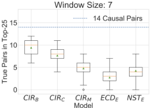
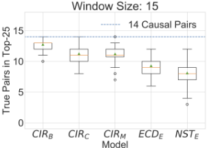
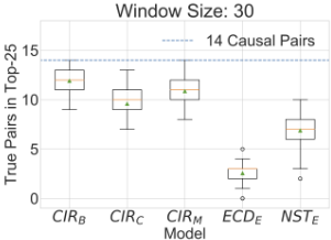
Figure 2 shows the distribution of performance over all 100 datasets for our methods at recovering the true causal pairs from the 40P2 = 380 event pairs; this is Hits@K which is a common metric in information retrieval [Baeza-Yates and Ribeiro-Neto, 2011]. Since our methods provide a score for each causal pair, we can use these to rank potentially causal pairs. The graphs show the counts of the true causal pairs in the top-25 scoring pairs for each of our scores over the 100 traces generated. We observe that across all window sizes, the intensity-based scores strictly dominate ECDE and NSTE scores. This provides evidence that our CIR scores provide a robust indication of the causal pairs on a timeline. More encouragingly, for windows 15 and 30 we see that the CIR models are able to surface all true causal pairs in the top-25. We suspect CIRB performs better than CIRM here because the synthetic dataset generation uses sparse graphs with only excitatory effects; a simple comparison to base rate (without accounting for other effects) therefore performs well.
| Method | K = 10 | K = 15 | K = 20 |
|---|---|---|---|
| CIRB | 4 | 6 | 6 |
| CIRC | 3 | 3 | 5 |
| CIRM | 6 | 7 | 7 |
| ECDE | 2 | 1 | 1 |
| NSTE | 5 | 4 | 7 |
5 Experiments on a Diabetes Event Dataset
We compare the methods/scores on a dataset with information pertaining to blood glucose levels, insulin dosage, eating and exercise patterns of 70 diabetes patients [Frank and Asuncion, 2010]. We follow Acharya [2014] and convert the data for each patient into an event dataset, treating expert assessments in that work as ground truth. A complication is that the assessments were conducted by assuming that the underlying causal graph is acyclic, which is not necessarily true for event pairs because both (x, y) and (y, x) could be causal; as a result, we are confident that the 11 pairs assessed to be causal are truly causal but suspect there are other causal associations that were missed.
We split the dataset into equal-sized training/test sets, determine a method's optimal hyper-parameter setting on the training set, and then compute the Hits@K on the test set using this hyper-parameter setting. The following hyperparameter settings were used during training: α ∈ {0, 1, 5}, λ ∈ {0, 0.5, 1} for NSTE, γ ∈ {0.001, 0.01, 0.1} for ECDE, g = {avg,max,min} for CIRM and window w = {0.1, 0.3, 0.5, 1} days for all models.
Table 1 compares the Hits@K across the five methods on the test set for K = 10, 15, 20, illustrating that CIRM performs best on this dataset. Note that it is possible for a method's Hits@K to decrease with K here as different hyperparameter setting may be chosen while optimizing over the training set. Since CIRM first requires learning a graph before aggregation (unlike the other models), we recommend learning a single graph using all independent event streams, when available like in this case, rather than learning a separate graph for each event stream and then aggregating pairwise scores. Here, both approaches yield identical results.
6 Experiments on a Political Event Dataset
Event datasets such as the Global Database of Events, Language and Tone (GDELT) [Leetaru and Schrodt, 2013] and the Integrated Crisis Early Warning System (ICEWS) [O'Brien, 2010] are popular in political science. Events in these datasets have a source actor performing an action on a target actor. Actors and actions in both ICEWS and GDELT are coded according to the Conflict and Mediation Event Observations (CAMEO) ontology which includes a host of domestic and international actor types. We use a subset of ICEWS in our experiments, including events over 10 years in 3 countries: Argentina, Mexico, and Venezuela, ending up with ∼25K event records spanning ∼2K distinct event types. Actor-BasedConditions. For these experiments, we investigate the use of supporting knowledge in conjunction with statistical co-occurrence of events for potential causal discovery. We conjecture that imposing additional conditions based on actor identities could enforce causal knowledge and thereby potentially match human assessments of causality. We refer to one such condition as the common actor condition: event pairs with a common actor are more amenable to be assessed by humans as causal. This notion has been explored in other contexts [Chambers and Jurafsky, 2008]. Requiring a common actor between events could model retaliation, reciprocity and reinforcement. We also consider a foreign actor condition: a foreign actor cannot influence an event between domestic actors. This reinforces the locality of events.
Surveys. To obtain benchmark causal relationships from our dataset, we designed surveys with 100 questions each for the 3 Latin American countries. To construct the surveys, we drew 25 pairs, uniformly at random, from each quartile of the ranked NSTE scores for each country. We did this to ensure the presence of some pairs that are suspected to be causal and some that are not. The surveys were provided independently to six project members with two countries each, resulting in three raters for each question. Participants were asked whether the question involved a plausible causal pair of events (yes/no) and to also specify how confident they were about their answer (0 - 100%). All three raters were unanimous in their decision for a majority of the questions (225/400 questions). We observe good pairwise agreement between the raters (≥ 0.68) for all countries.
Confidence Strength Task. We aggregate the human assessments about confidence into a numeric confidence strength which we predict using a linear regression model on the cause-effect scores (after z-scoring). This strength is measured on a scale of -1 (strong no) to 1 (strong yes) and obtained by applying a +ve (-ve) sign for the binary response yes (no) and averaging over raters' confidences, e.g., three raters' responses with confidences are {(no, 70%), (no, 40%), (yes, 50%)}, the confidence strength is (-0.7 - 0.4 + 0.5)/3 = -0.2. We use negative root mean squared error as the evaluation metric (higher is better). As there are 20 questions that are tested in every fold, the potential range for this metric is 0 (best) to -2√20 ≈ -9 (worst), which occurs if for all questions in all folds, a strength of -1 (strong no) is predicted to be 1 (strong yes) or vice-versa.
Table 2 compares this metric across the folds for the 3 countries, as a function of the imposed actor conditions.The conditional intensity based scores (particularly CIRM but also CIRB) generally perform the best on this task. We observe that imposing the actor based conditions improves performance in many cases. Overall, the small mean errors observed in this task (relative to the scale) indicate that the scores are good at predicting the numeric confidence strength.
| Condition | Argentina | Mexico | Venezuela |
|---|---|---|---|
| Neither | -0.37 (ECDE) | -0.19 (CIRM) | -0.32 (CIRM) |
| Common Actor | -0.37 (ECDE) | -0.17 (CIRM) | -0.33 (CIRM) |
| Foreign Actor | -0.32 (CIRB) | -0.19 (CIRM) | -0.28 (ECDE) |
| Both | -0.35 (CIRB) | -0.17 (CIRM) | -0.3 (CIRB) |
7 Conclusions
We proposed several scores for discovering causal association between pairs of events from event datasets, including a general framework that subsumes the proposed scores and that could be useful for future advances. The conditional intensity based scores are a major contribution in this work. They are mathematically principled for continuous-time data and perform well on synthetic datasets as well as two real-world datasets. We demonstrated, through an evaluation benchmark constructed with political events, that incorporating actorbased information in addition to statistical associations could help with matching human causal assessment for relational events. Investigating more complex causal scoring functions and studying their efficacy and interpretability across a variety of event datasets is a potential direction for future work, as is a principled approach to learn the window parameter w.
Data-driven AI systems that assist analysts with long-term and wide ranging future possibilities need sufficiently rich knowledge about causal relationships between events. Discovering such relationships using statistical associations remains a challenging but worthy endeavor, in our opinion. Our work complements the current literature towards endowing these systems with such knowledge.
Acknowledgments
We would like to thank Oktie Hassanzadeh and Shari Trewin for their help with this project, as well as the anonymous reviewers, who helped improve the paper.
@inproceedings{ijcai2020p167,
  title     = {Cause-Effect Association between Event Pairs in Event Datasets},
  author    = {Bhattacharjya, Debarun and Gao, Tian and Mattei, Nicholas and Subramanian, Dharmashankar},
  booktitle = {Proceedings of the Twenty-Ninth International Joint Conference on
               Artificial Intelligence, {IJCAI-20}},
  publisher = {International Joint Conferences on Artificial Intelligence Organization},
  editor    = {Christian Bessiere},
  pages     = {1202--1208},
  year      = {2020},
  month     = {7},
  note      = {Main track},
  doi       = {10.24963/ijcai.2020/167},
  url       = {https://doi.org/10.24963/ijcai.2020/167},
}
TY - CPAPER TI - Cause-Effect Association between Event Pairs in Event Datasets AU - Bhattacharjya, Debarun AU - Gao, Tian AU - Mattei, Nicholas AU - Subramanian, Dharmashankar T2 - Proceedings of the Twenty-Ninth International Joint Conference on Artificial Intelligence, IJCAI-20 PB - International Joint Conferences on Artificial Intelligence Organization PY - 2020 SP - 1202 EP - 1208 DO - 10.24963/ijcai.2020/167 UR - https://doi.org/10.24963/ijcai.2020/167 ER -Copied
Machine-readable versions of this paper, for tools and AI agents:





