
Bipartite Encoding: A New Binary Encoding for Solving Non-Binary CSPs
Proceedings of the Twenty-Ninth International Joint Conference on Artificial Intelligence. Main track. Pages 1184-1191.
https://doi.org/10.24963/ijcai.2020/165
Keywords
- Constraints and SAT: Constraint Satisfaction
- Constraints and SAT: Constraints: Modeling, Solvers, Applications
Abstract
Constraint Satisfaction Problems (CSPs) are typically solved with Generalized Arc Consistency (GAC). A general CSP can also be encoded into a binary CSP and solved with Arc Consistency (AC). The well-known Hidden Variable Encoding (HVE) is still a state-of-the-art binary encoding for solving CSPs. We propose a new binary encoding, called Bipartite Encoding (BE) which uses the idea of partitioning constraints. A BE encoded CSP can achieve a higher level of consistency than GAC on the original CSP. We give an algorithm for creating compact bipartite encoding for non-binary CSPs. We present a AC propagator on the binary constraints from BE exploiting their special structure. Experiments on a large set of non-binary CSP benchmarks with table constraints using the Wdeg, Activity and Impact heuristics show that BE with our AC propagator can outperform existing state-of-the-art GAC algorithms (CT, STRbit) and binary encodings (HVE with HTAC).
- [Bessiere et al., 2008] Christian Bessiere, Kostas Stergiou, and Toby Walsh. Domain filtering consistencies for non- binary constraints. Artificial Intelligence, 172(6-7):800- 822, 2008.
- [Boussemart et al., 2004] Frédéric Boussemart, Fred Hemery, Christophe Lecoutre, and Lakhdar Sais. Boost- ing systematic search by weighting constraints. In European Conference on Artificial Intelligence, 2004.
- [Briggs and Torczon, 1993] Preston Briggs and Linda Torc- zon. An efficient representation for sparse sets. ACM Let- ters on Programming Languages and Systems (LOPLAS), 2(1-4):59-69, 1993.
- [Dechter and Pearl, 1989] Rina Dechter and Judea Pearl. Tree clustering for constraint networks. Artificial Intel- ligence, 38(3):353-366, 1989.
- [Demeulenaere et al., 2016] Jordan Demeulenaere, Renaud Hartert, Christophe Lecoutre, Guillaume Perez, Laurent Perron, Jean-Charles Régin, and Pierre Schaus. Compact- Table: efficiently filtering table constraints with reversible sparse bit-sets. In International Conference on Principles and Practice of Constraint Programming, 2016.
- [Dolan and Moré, 2002] Elizabeth D Dolan and Jorge J Moré. Benchmarking optimization software with perfor- mance profiles. Mathematical programming, 91(2):201- 213, 2002.
- [Janssen et al., 1989] Philippe Janssen, Philippe Jégou, Bernard Nouguier, and Marie-Catherine Vilarem. A fil- tering process for general constraint-satisfaction problems: achieving pairwise-consistency using an associated binary representation. In IEEE International Workshop on Tools for Artificial Intelligence, 1989.
- [Lecoutre and Szymanek, 2006] Christophe Lecoutre and Radoslaw Szymanek. Generalized arc consistency for pos- itive table constraints. In International Conference on Principles and Practice of Constraint Programming, 2006.
- [Lecoutre and Vion, 2008] Christophe Lecoutre and Julien Vion. Enforcing arc consistency using bitwise operations. Constraint Programming Letters, 2:21-35, 2008.
- [Lecoutre et al., 2012] Christophe Lecoutre, Chavalit Likit- vivatanavong, and Roland H.C. Yap. A path-optimal GAC algorithm for table constraints. In European Conference on Artificial Intelligence, 2012.
- [Lecoutre et al., 2013] Christophe Lecoutre, Anastasia Pa- parrizou, and Kostas Stergiou. Extending STR to a higher- order consistency. In AAAI Conference on Artificial Intel- ligence, 2013.
- [Lecoutre, 2011] Christophe Lecoutre. STR2: optimized simple tabular reduction for table constraints. Constraints, 16(4):341-371, 2011.
- [Likitvivatanavong et al., 2014] Chavalit Likitvivatanavong, Wei Xia, and Roland H.C. Yap. Higher-order consisten- cies through GAC on factor variables. In International Conference on Principles and Practice of Constraint Pro- gramming, 2014.
- [Michel and Van Hentenryck, 2012] Laurent Michel and Pascal Van Hentenryck. Activity-based search for black- box constraint programming solvers. In International Conference on Integration of Artificial Intelligence and Operations Research Techniques in Constraint Programming, 2012.
- [Refalo, 2004] Philippe Refalo. Impact-based search strate- gies for constraint programming. In International Confer- ence on Principles and Practice of Constraint Program- ming, 2004.
- [Rossi et al., 1990] Francesca Rossi, Charles J Petrie, and Vasant Dhar. On the equivalence of constraint satisfaction problems. In European Conference on Artificial Intelli- gence, 1990.
- [Samaras and Stergiou, 2005] Nikolaos Samaras and Kostas Stergiou. Binary encodings of non-binary constraint sat- isfaction problems: Algorithms and experimental results. Journal of Artificial Intelligence Research, 24:641-684, 2005.
- [Schneider and Choueiry, 2018] Anthony Schneider and Berthe Y Choueiry. PW-CT: extending Compact-Table to enforce pairwise consistency on table constraints. In International Conference on Principles and Practice of Constraint Programming, 2018.
- [Smith and Grant, 1998] Barbara M Smith and Stuart A Grant. Trying harder to fail first. In European Conference on Artificial Intelligence, 1998.
- [Stergiou and Walsh, 1999] Kostas Stergiou and Toby Walsh. Encodings of non-binary constraint satisfac- tion problems. In National Conference on Artificial Intelligence, 1999.
- [Verhaeghe et al., 2018] Hélene Verhaeghe, Christophe Lecoutre, and Pierre Schaus. Compact-MDD: Efficiently filtering (s)MDD constraints with reversible sparse bit-sets. In International Joint Conference on Artificial Intelligence, 2018. IJCAI
- [Verhaeghe et al., 2019] Hélène Verhaeghe, Christophe Lecoutre, and Pierre Schaus. Extending Compact- Diagram to basic smart multi-valued variable diagrams. In International Conference on Integration of Constraint Programming, Artificial Intelligence, and Operations Research, 2019.
- [Wang and Yap, 2019] Ruiwei Wang and Roland H.C. Yap. Arc consistency revisited. In International Conference on Integration of Constraint Programming, Artificial Intelli- gence, and Operations Research, 2019.
- [Wang et al., 2016] Ruiwei Wang, Wei Xia, Roland H.C. Yap, and Zhanshan Li. Optimizing simple tabular reduc- tion with a bitwise representation. In International Joint Conference on Artificial Intelligence, 2016. IJCAI
- [Yap et al., 2020] Roland H.C. Yap, Wei Xia, and Ruiwei Wang. Generalized arc consistency algorithms for table constraints: A summary of algorithmic ideas. In AAAI Conference on Artificial Intelligence, 2020.
References were extracted automatically from the PDF and may contain errors.
Full text extracted automatically from the PDF; figures, tables and equations may differ. The PDF is the version of record.
1 Introduction
Many combinatorial problems from AI can be naturally modelled as Constraint Satisfaction Problems (CSPs) with constraints. Typically solving a (non-binary) CSP uses Generalized Arc Consistency (GAC) on the (non-binary) constraints. Alternatively, a non-binary CSP can be transformed with binary encoding into a CSP with only binary constraints so that Arc Consistency (AC) is applicable. While AC is simpler than GAC and binary encodings are well known, it is only recently that solving with binary encoding is shown to be practical. The hidden variable encoding with the AC algorithm HTAC [Wang and Yap, 2019] was shown to be competitive with state-of-the-art GAC algorithms on non-binary CSPs.
Bit representation is the key to the efficiency of many stateof-the-art GAC/AC algorithms for table constraints. A recent survey describes improvements in GAC algorithms [Yap et al., 2020]). Here, we summarize some recent GAC algorithms and ideas. Bit sets are used to represent variable domains in AC3bit [Lecoutre and Vion, 2008]. GAC algorithms STRbit [Wang et al., 2016] and CT [Demeulenaere et al., 2016] optimize the simple tabular reduction algorithms
[Lecoutre, 2011; Lecoutre et al., 2012] representing constraint relations as bit sets. Recently, bit representation were extended to handle compact representations and high-order consistencies. However, experiments show that the CT algorithm is still overall faster than these newer algorithms (see the experimental results of PW-CT [Schneider and Choueiry, 2018], compact-MDD [Verhaeghe et al., 2018] and smart MDD [Verhaeghe et al., 2019]).
The hidden variable encoding (HVE) [Rossi et al., 1990], dual encoding [Dechter and Pearl, 1989] and double encoding [Stergiou and Walsh, 1999] are well known binary encodings for reducing non-binary CSPs to binary CSPs. AC on a HVE instance achieves GAC on the original CSP but is weaker than AC on the dual/double encoding instance [Bessiere et al., 2008]. However, the drawback is that dual/double encoding instances may be much larger than HVE instances. HVE, proposed 30 years ago, is the state-of-the-art binary encoding [Wang and Yap, 2019]. We observe that binary encoding instances have special structure. Specialized AC algorithms, such as HAC, PW-AC [Samaras and Stergiou, 2005] and HTAC have been proposed to handle binary encoded instances. In particular, HTAC is competitive with CT, suggesting that AC algorithms on binary encoded instances have the potential to outperform the state-of-the-art GAC algorithms.
In this paper, we propose a new binary encoding, called bipartite encoding (BE), which encodes constraints as binary constraints between factor variables which partition the constraint scopes. AC on a BE encoded CSP is stronger than GAC on the original CSP. We give an algorithm to construct BE instances, followed by a AC propagator AC-BE which treats a connected component in the binary encoding as a "special constraint". We evaluate the bipartite encoding to solve non-binary CSPs comparing with state-of-the-art GAC algorithms and the binary encoding HVE (with HTAC) on a large set of benchmarks. The results show that the BE propagator outperforms CT, STRbit and HTAC across many variable heuristics (Wdeg, Activity, Impact). The usefulness of higher consistency is also shown to be effective making some instances backtrack free.
The remainder of the paper is organized as follows. Section 2 provides preliminaries. The bipartite encoding, an algorithm to create BE instances and a special propagator for BE are given in Sections 3, 4 and 5. Experiments are presented in Section 6 and Section 7 concludes.
x1 x2 x5 x6
2 Preliminaries
A CSP P is a pair (X, C) where X = {x1, x2, . . . , xn} is a set of n variables, D(xi) is the domain of variable xi, and C = {c1, c2, . . . , ce} is a set of e constraints. In this paper, we assume that D(x) is finite, also known as finite domain. A literal of a variable x is a variable value (x, a). A tuple over a set of variables {xi1 , xi2 , . . . , xir } is a set of literals {(xi1 , a1), (xi2 , a2), . . . , (xir , ar)}. Each constraint cj consists of a constraint scope scp(cj) ⊆ X and a relation rel(cj) which is defined by a set of tuples over scp(cj). The arity of constraint c is the number of variables in the constraint scope, i.e. |scp(c)|. P is a r-arity CSP if the largest constraint arity is r. A 2-arity CSP is also called a binary CSP. Without loss of generality, all 1-arity constraints are removed by modifying variable domains. A non-binary CSP is a r-arity CSP where r > 2. We assume the CSP is normalized, i.e. for each constraint ci ∈ C such that scp(ci) ⊆ scp(cj), ci is removed by joining ci with cj .
The projection of a tuple τ (or a set T of tuples) on a set S of variables, denoted by τ [S] (or T [S]), is {(x, a) ∈ τ |x ∈ S} (or {τ[S]|τ ∈ T}). A tuple τ is valid iff for all literals (x, a) ∈ τ, the value a is in D(x) and x only appears once in τ. A tuple τ over variables X ⊆ X is consistent iff τ[scp(c)] ∈ rel(c) for all constraints c ∈ C such that scp(c) ⊆ X. A solution of P is a consistent and valid tuple over X. P is satisfiable iff there is a solution over X. A support of a value a ∈ D(x) on a constraint c is a tuple τ ∈ rel(c) such that (x, a) = τ[x]. A support of a tuple τ1 ∈ rel(ci) on a constraint cj is a tuple τ2 ∈ rel(cj) such that τ2[scp(ci)] = τ1[scp(cj)]. For binary CSPs, b ∈ D(y) is a support of a ∈ D(x) on y if the tuple {(x, a), (y, b)} is a support of a on the constraints between x and y.
A variable x ∈ scp(ci) is Generalized Arc Consistent (GAC) on a constraint ci ∈ C if a has a valid support on ci for all a ∈ D(x). A constraint ci is GAC if all variables in scp(ci) are GAC on ci. A CSP (X, C) is GAC if all constraints in C are GAC. For binary CSPs, GAC is also called Arc Consistent (AC). GAC is a first-order consistency, filtering variable domains. We also introduce a higherorder consistency to further filter inconsistent tuples. A tuple τ ∈ rel(ci) is Pairwise Consistent (PWC) if τ has a valid support on cj for all cj ∈ C [Janssen et al., 1989]. A constraint ci is PWC if all tuples τ ∈ rel(ci) are PWC. A CSP (X , C) is PWC if all constraints in C are PWC. A CSP P is Full Pairwise Consistent (FPWC) if P is PWC and GAC [Lecoutre et al., 2013; Likitvivatanavong et al., 2014].

3 Bipartite Encoding
We start with an observation that in a binary CSP, every binary constraint is between two variables which partition the constraint scope. So we can think of a binary CSP as being encoded with such a partitioning. We generalize this idea of encoding to a new binary encoding of non-binary CSPs called bipartite encoding which can also give stronger consistency than GAC.
Definition 1. Given a CSP P = (X , C), a factor variable fv over a non-empty set of variables S ⊆ X is a new variable such that D(fv) is a set of tuples over S, and τ[S] ∈ D(fv) for all solutions τ of P. We use scp(fv) = S to denote the scope of the variables covered by fv. A factor variable fv is original if |scp(fv)| = 1 and compound if |scp(fv)| > 1.
The minimum domain of a factor variable fv consists of all tuples τ over scp(fv) which can be extended to solutions of the CSP. As such, it is NP-hard to find the minimum domain of fv. We propose to use some local consistent tuples to construct D(fv).
Definition 2. A bipartite encoding BE(P) of a CSP P = (X , C) is a CSP (X + ∪ X ∗ , C+ ∪ C ∗ ), where
- Variables are either compound or original factor variables denoted by X ∗ and X + respectively and for all variables fvi, fvj ∈ X ∗ ∪X +, scp(fvi) ̸= scp(fvj) if i ̸= j.
- Partition constraints C ∗ : for each ci ∈ C, c∗i ∈ C ∗ is a binary constraint such that scp(c∗i )={fvj, fvk}, {scp(fvj), scp(fvk)} is either a disjoint or non-disjoint partition of scp(ci), and rel(c∗i )={{τ1, τ2}|τ1 ∈ D(fvj), τ2 ∈ D(fvk), (τ1 ∪ τ2) ∈ rel(ci)}.
- Mapping constraints C+: for each fvi ∈ X ∗ and x ∈ scp(fvi), cxi ∈ C+ is a binary constraint such that scp(cxi ) = {fvi, fvj}, scp(fvj) = {x}, and rel(cxi ) = {{τ1, τ2}|τ1 ∈ D(fvj), τ1 ∈ D(fvj), τ2 = τ1[scp(fvj)]}.
For all factor variables fvi, the information of the tuples in the domain D(fvi) is recorded in the mapping constraints {cxi |x ∈ scp(fvi)}, which ensures that the tuple τ1 ∪ ... ∪ τm is an assignment of P if the tuple {(fv1, τ1),...(fvm, τm)} is consistent on BE(P). We remark that the mapping constraints used are similar to the constraints in HVE encoding and there may be other mapping constraints ensuring the same property. Additionally, for each partition constraint c∗i ∈ C ∗ , all tuples {(fvj, τ1), (fvk, τ2)} in rel(c∗i ) correspond to the tuples τ1 ∪ τ2 in rel(ci), which ensures that the tuple τ1 ∪ ... ∪ τm is a solution of P if the tuple (fv1, τ1),...(fvm, τm)} is a solution of BE(P).
Algorithm 1: BE(X ,C)
1 scpp ← partition(C); S ← (⋃ci∈C scpp[ci]) ∪ (⋃x∈X {{x}}); 2 V ← ∅; for Sj ∈ S do Generate a factor variable fvj & domain on Sj ; 3 V ← V ∪ {fvj}; 4 C ∗ ← ∅; for ci ∈ C do {Sj , Sk}← scpp[ci]; Construct a constraint c∗i between fvj and fvk; C ∗ ← C ∗ ∪ {c∗i }; 5 Construct constraints C+ with factor variables in V ;- return (V, C ∗ ∪ C+);
Example 1. Let CSP P=(X, C) where C={c1, c2}, X={x1, · · · , x6} and domains are {0,1}. Constraint scopes are: scp(c1)={x1, · · · , x4} and scp(c2)={x1, x2, x5, x6} with relations given in Figure 1a, 1b. A bipartite encoding ({fv1, fv2, fv3, xf1 , · · · , xf6 }, {c∗1 , c∗2 , cx1 1 , · · · , cx6 3 }) of P is shown in Figures 1c,· · · ,1j. Constraints c1 and c2 are represented as c∗1 and c∗2 , where scp(c∗1 ) = {fv1, fv2} and scp(c∗2 ) = {fv1, fv3}. fv1, fv2 and fv3 are compound factor variables on S1 = {x1, x2}, S2 = {x3, x4} and S3 = {x5, x6}. xfi is an original factor variable over {xi} for 1 ≤ i ≤ 6. For each factor variable on {x, y}, we use values 0, 1, 2 and 3 to denote tuples {(x, 0), (y, 0)}, {(x, 0), (y, 1)}, {(x, 1), (y, 0)} and {(x, 1), (y, 1)}, respectively. For each original factor variable xfi , value a denotes {(xi, a)}. Each solution of BE(P) corresponds to a solution of P, e.g. {(fv1, 0), (fv2, 1), (fv3, 3), (xf1 , 0), (xf2 , 0), (xf3 , 0), (xf4 , 1), (xf5 , 1), (xf6 , 1)} corresponds to {(x1, 0), (x2, 0), (x3, 0), (x4, 1), (x5, 1), (x6, 1)}.
For a bipartite encoding BE(P) = (X ∗ ∪ X +, C ∗ ∪ C+), every original factor variable in X + (or constraint in C ∗ ) corresponds to a variable (or constraint) in P. An image P ′ of BE(P) is a CSP (X ′ , C ′ ) such that X ′ = {x′ |x ∈ X} and C ′ = {c′i |ci ∈ C}, where D(x′ )={a|(x, a) ∈ D(xf )}, scp(c′i ) = {x′ |x ∈ scp(ci)} and rel(c′i ) = {{(x′ , a)|(x, a) ∈ τ1 ∪τ2} | {(fvj , τ1), (fvk, τ2)} ∈ rel(c∗i )}. The image P ′ of BE(P) has the same variables and constraints as P, except the domains and relations of P ′ may be reduced. P ′ is useful for comparing the consistencies on BE(P) with that on P.
Proof. Assume scp(c∗i ) = {fvj, fvk}, |scp(fvj)| > 1, x ∈ scp(fvj), and a ∈ D(x′ ). BE(P) is AC, hence, (xf , {(x, a)}) has a valid support on τ1 ∈ D(fvj) and τ1 has a valid support τ2 ∈ D(fvk). So {(y′ , b)|(y′ , b) ∈ τ1 ∪ τ2} is a valid support of (x′ , a) on c′j .
AC on BE(P) can be stronger than GAC on P (see Proposition 2). For example, (xf1 , 1) is not AC on the BE instance given in Figure 1, but the original CSP is GAC.
Algorithm 2: partition(C)
cur ← C; while cur ̸= ∅ do 1 E ←maxEdge(cur); if E = ∅ then break; 2 for {ci, cj} ∈ E do Sk ← scp(ci) ∩ scp(cj ); scpp[ci] ← {Sk, scp(ci) \ Sk}; 3 scpp[cj ] ← {Sk, scp(cj ) \ Sk}; 4 for ci ∈ cur do Select a variable x from scp(ci); 5 scpp[ci] = {scp(ci) \ {x}, {x}}; return scpp;Algorithm 3: maxEdge(cur)
- Let E be all maximum edges in cur; S ← {scp(ci) ∩ scp(cj )|{ci, cj } ∈ E}; for Sk ∈ S do 1 size[Sk] ← domain size of a factor variable on Sk; 2 N[Sk] ← ⋃{e ∈ E|e ⊆ cur, scp(e) = Sk}; Er ← ∅; while S ̸= ∅ do 3 Let M be the maximum cardinality subsets in S; 4 Select Sk fromM such that size[Sk] |N[Sk]| is minimum; S ← S \ {Sk}; 5 A← {c ∈ (N[Sk] ∩ cur)| c is size splittable by Sk}; EA ← {e ∈ E|scp(e) = Sk, e ⊆ A}; 6 Er ←Er ∪EA; cur ← cur \ (⋃e∈EA e);
return Er ;
4 A Bipartite Encoding Algorithm
We present Algorithm 1 for constructing a bipartite encoding instance from a CSP (X, C). It is based on partitions of constraint scopes and has three parts given in Algorithm 1:
- (i) For each constraint ci ∈ C, the partition function split scps(ci) into 2 subsets scpp[ci] (Line 1-see Sec. 4.1).
- (ii) Generating factor variables (Lines 2-3). We use the projection ⋂{rel(c)[scp(fv)]|c ∈ C, scp(fv) ⊆ scp(c)} as the domain of a factor variable fv, and remove invalid tuples from constraint relations after generating each factor variable, e.g. for the CSP in Figure 1, we can remove the tuple {(x1, 1), (x2, 1), (x5, 0), (x6, 0)} from rel(c2) after generating the factor variable fv1 on {x1, x2}. As {(x1, 1), (x2, 1)} is removed, then {(x5, 0), (x6, 0)} is not included in the domain of the factor variable fv3 on {x5, x6}.
- (iii) Constructing bipartite encoding instance based on the generated factor variables and partitions of constraint scopes (Lines 4-5)-this is a straightforward construction using Definition 2.
The number of possible partitions of constraint scopes is exponential in the number of constraints and constraint arity. Thus, many BE instances can be constructed for a CSP by applying different partitions. We introduce a heuristic used to generate some disjoint partitions in the following subsection.
4.1 MaximumEdge Partition
We now give a method to partition the non-binary constraints taking into account obtaining higher level consistency where feasible. We first introduce some notations. A dual graph [Dechter and Pearl, 1989] of a CSP P = (X, C) is a undirected graph such that constraints C are nodes and edges are {{ci, cj} ⊆ C|scp(ci) ∩ scp(cj) ̸= ∅}. We use scp(e) = scp(ci) ∩ scp(cj) to denote the scope of variables covered by a edge e = {ci, cj}. The size of an edge e is the cardinality of scp(e). The edge e = {ci, cj} is a maximum edge of ci in C ⊆ C if the size of e is greater than 1 and largest on all edges in C including ci, and e is a maximum edge in C if e is a maximum edge of ci or cj in C. A bipartite encoding BE(P) covers an edge e = {ci, cj} if there exists a factor variable fv in scp(c∗i )∩scp(c∗j ) such that scp(fv) = scp(e), e.g. the bipartite encoding given in Figure 1 covers the edge {c1, c2}, since scp(c∗1 ) ∩ scp(c∗2 ) includes a factor variable fv1 on {x1, x2}. Our strategy is that for overall propagation efficiency, the size of the encoding should be compact, in particular, we will focus on bit representations used in GAC/AC propagators. We propose a bipartite encoding heuristic where the encoding is compact and can cover some maximum edges for higher level consistency (see Proposition 2).
Proposition 2. The image P ′ of BE(P) is FPWC if BE(P) is AC and covers all edges whose sizes are greater than 1.
Proof. For all c′i , c′j ∈ C ′ and τ ∈ rel(c′i ) such that S = scp(ci) ∩ scp(cj) includes at least 2 variables, τ has a valid support on c′j , since τ[S] is in D(fvk) and has valid supports on c∗j , where fvk ∈ scp(c∗i ) ∩ scp(c∗j ) is a factor variable on S. Recall, P ′ is AC (Proposition 1), so P ′ is FPWC.
Algorithm 2 generates partitions of constraint scopes. The data structure scpp[ci] records the partition of scp(ci). Algorithms 2 and 3 use a global set cur to record a set of constraints which are not partitioned. At Line 1, Algorithm 3 is called to generate a subset E of maximum edges in cur such that: (i) for each ci ∈ cur, there is at most one partition of scp(ci) based on E, i.e. |{scp(e)|e ∈ E, ci ∈ e}| ≤ 1; and (ii) for each edge e = {ci, cj} in E, the constraints ci and cj are size splittable by scp(e). If E is not empty, we use the maximum edges in E to partition some constraint scopes (Lines 2-3), otherwise we use a basic partitioning-for each constraint ci in cur, we select the last variable x in scp(ci) and partition scp(ci) (between Lines 4 and 5).
A constraint ck is size splittable by a variable subset Si ⊂ scp(ck) or Sj = scp(ck) \ Si if the size of the bit representation (see data structures used in HTAC [Wang and Yap, 2019]) of ck is greater than or equal to that of the corresponding constraints in the BE encoding, namely, the sum of the sizes of the binary constraints c∗k and {cxl ∈ C+|scp(fvl) ∈
{Si, Sj}, x ∈ scp(fvl)}. 1 We propose to evaluate the size of the original and bipartite instance as follows. We use |rel(ck)|(∑x∈scp(ck) |D(x)|) to evaluate the size of the bit representation of ck. For each binary constraint in the BE encoding, we use |D(fvl1 )| × |D(fvl2 )| to estimate the size of the constraint, where {fvl1 , fvl2 } is the constraint scope.
Algorithm 3 gives our maximum edges generation algorithm. The data structure size[Sk] records the domain size of the factor variable fvk on Sk (at Line 1). At Line 2, N[Sk] is a set of constraints where the constraint scopes may be partitioned by Sk. At Lines 3 and 4, we first select a variable subset Sk from S with maximum cardinality, and further select those with minimum size[Sk] N[Sk] . Lines 5-6 evaluate which constraints in N[Sk] are size splittable by Sk, recording the corresponding maximum edges in Er. We remark that we also delete some invalid tuples when calculating the domain size of a factor variable.
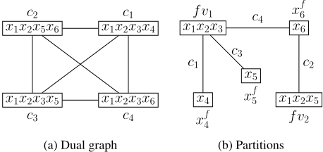
Example 2. Let P be a CSP with constraints {c1, · · · , c4}, variables {x1, · · · , x6} and domains {0, 1}. c1, c2, c3 and c4 are the linear equations: x1+x2+x3+x4=1, x1+x2+x5+ x6=2, x1+x2+x3+x5=2 and x1+x2+x3+x6=1. Figure 2a is the dual graph of P. Figure 2b gives the partitions generated by our algorithm. There are 5 maximum edges, the scopes are S1={x1, x2, x3}, S2={x1, x2, x5} and S3={x1, x2, x6} with N[S1]={c1, c3, c4}, N[S2]={c2, c3} and N[S3]={c2, c4}. We generate the factor variables on S1, S2 and S3, and then record the corresponding domain sizes. At Line 4 in Algorithm 3, S1 is selected. c1, c3 and c4 are size splittable by S1, thus, {c1, c3}, {c1, c4} and {c3, c4} are the maximum edges selected. Then {S1, {x4}}, {S1, {x5}} and {S1, {x6}} are the partitions of scp(c1), scp(c3) and scp(c4). After partitioning c1, c3 and c4, there are no more maximum edges, so we select x6 from scp(c2), with partition of scp(c2) being {{x1, x2, x5}, {x6}}. Then we construct a BE instance (X ∗ ∪ X +, C ∗ ∪ C+) such that X ∗={fv1, fv2}, X +={xf1 , xf2 , xf3 , xf4 , xf5 , xf6 }, C ∗={c∗1 , c∗2 , c∗3 , c∗4 }, and C+={cx1 1 , cx2 1 , cx3 1 , cx1 2 , cx2 2 , cx5 2 }, where scp(fv1)=S1, scp(fv2)=S2, scp(xfi )={xi} for 1 ≤ i ≤ 6, scp(c∗1 )={fv1, xf4 }, scp(c∗2 )={fv2, xf6 }, scp(c∗3 )={fv1, xf5 } and scp(c∗4 )={fv1, xf6 }.
1 We remark that experiments show HTAC on the HVE encoding is competitive with CT on the original CSP, and as the experiments show, we want to improve on both. This means that attention is also needed on the size of the bit representations of the constraints.
5 AC on Bipartite Encoding Instances
HTAC is a state-of-the-art specialized AC algorithm for nonbinary CSPs encoded by HVE. It exploits the structure of the binary CSP arising from the encoding- the set of binary constraints from encoding a non-binary constraint is regarded as a special subset of the constraints in HVE instance. Correspondingly, a specialized propagator AC-H is used for each subset with a star structure in the constraint graph. HTAC only needs to search on the original variables.
A BE instance is a binary CSP so any AC algorithm can be applied. However, in the same way that HTAC uses a specialized propagator, our AC-BE algorithm is a specialized propagator exploiting the structure of a BE instance (X + ∪ X ∗ , C+ ∪ C ∗ ) extending the framework of HTAC. We partition binary constraints in the BE instance into a set of connected components in an undirected graph (C1,E), and employ special propagators for the components, where C1 = C+∪C ∗ and E = {{ci, cj} ⊆ C1|scp(ci)∩scp(cj )∩X ∗ ̸= ∅}, and every component is treated as a set of constraints. Meanwhile, we also only search on the original factor variables in X +. Due to lack of space, we refer readers to [Wang and Yap, 2019] for details on algorithms and data structures in HTAC.
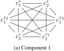
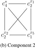
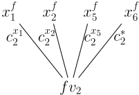
Example 3. There are 2 connected components for the BE instance given in Example 2. Figure 3a is the first component {cx1 1 , cx2 1 , cx3 1 , c∗1 , c∗2 , c∗3 }. The constraint scopes of all constraints in the first component include the factor variable fv1. Figure 3b shows the second component {cx1 2 , cx2 2 , cx5 2 , c∗4 }. The compound factor variable fv2 is included in the constraint scopes of all constraints in the second component. Note that the constraints in different components only share some original factor variables.
Algorithm 4: AC-BE(C)
V ← ⋃{scp(c)|c ∈ C}; 1 T ← ∅, U ←C; while ∃x ∈ V s.t. |{c ∈ U|x ∈ scp(c)}| = 1 do T ← T ∪ {c ∈ U|x ∈ scp(c)}; 2 U ←U \ {c ∈ U|x ∈ scp(c)}; 3 if ¬propagationUp(T) then return false ; 4 if ¬AC(U) then return false ; 5 if ¬propagationDown(T) then return false ; for x ∈ V ∩ X + s.t. D(x) is changed do 6 Add x to the propagation queue; return true;Every connected component C in the graph (C1,E) is regarded as a single "special constraint". Algorithm 4 presents a specialized propagation function for this component which enforces AC on all binary constraints in the component as follows. We first partition the binary constraints in C into two subsets T and U (between Lines 1 and 2) such that: (i) the primal graph of T is acyclic and (ii) every node in the primal graph of U is included in at least one cycle and (iii) every connected component in the primal graph of T has at most one node which is also included in the primal graph of U, where the primal graph of a set of binary constraints C ′ is a undirected graph (⋃c∈C′ scp(c), {scp(c)|c ∈ C ′ }). If U is empty, then the primal graph of C is acyclic, otherwise we have a special "star structure" such that the primal graph of U is the "root" and the trees included in the primal graph of T are the "leaves".
While an AC propagator can be used on the entire component C, we use a more efficient approach recognizing the tree structure in T. For the binary constraints in T, we call the revise functions to update the variable domains from leaves to the roots (the propagationUp function at Line 3), and then from roots to leaves (in the propagationDown function at Line 5), where for each connected component in the primal graph of T, a node is set as the root of the component, such that the nodes included in both the primal graphs of U and T are root nodes. For the binary constraints in U, we use a queue to record the variables which may cause reductions of other variable domains (same as the queue used in AC3bit ), and then iteratively propagate the variables in the queue (in the AC function at Line 4 which is a normal AC propagator). The propagationUp, propagationDown and AC functions employ some revise functions to update variable domains, and return false if there is a wipe-out of a domain, otherwise return true. At Line 6, if the domain of a variable x ∈ X + is changed, then x is added to a propagation queue shared by all connected components of the graph (C1,E), thus propagating to other constraints in C1.
Comparing to the normal AC propagators liking AC3bit , the specialized AC propagator for BE instances has a different propagation ordering which iteratively uses Algorithm 4 to enforce AC on a connected component of the graph (C1,E) until all connected components of (C1,E) are AC, where a connected component is AC if all binary constraints in the connected component are AC.
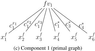
Example 4. Figure 3c and 3d shows the primal graph of the component given in Figure 3a and 3b respectively. Every edge in the primal graphs corresponds to a binary constraint in the BE instance. The primal graph of each component is acyclic and only includes one compound factor variable node. We set the compound factor variables as roots in the primal graphs. Correspondingly the propagationUp function updates the domains of compound factor variables (roots) based on the domains of original factor variables (leaves) and the propagationDown function updates the domains of leaves based on the domain of roots.
In our implementation, as common with the implementation of AC propagators, some revise functions are used. Our revise functions are based on those from HTAC which use the following functions to update a variable domain D(x) based on another variable domain D(y): (i) seekSupport scans all values in the domain D(x), removing values which do not have any valid support on y; (ii) reset updates D(x) by using the union of all supports on x of the values in D(y); and (iii) delete removes all supports on x of the values which are removed from D(y). For a binary constraint with scp(c) = {x, y}, our implementation uses the revise operations as follows. The seekSupport operation is used when x ∈ X + or |D(x)| ≤ |D(y)|. Otherwise, reset or delete operations are used to update the domain D(x). We use the delete operation as an optimization when the values in D(x) have at most 1 support in D(y). We adapt data structures employing sparse sets [Briggs and Torczon, 1993], sparse bit sets [Demeulenaere et al., 2016; Wang and Yap, 2019] and "ordered link" data structures [Lecoutre and Szymanek, 2006; Wang and Yap, 2019].
6 Experiments
Experiments presented in recent GAC algorithms (compactMDD, smart MDD and PW-CT (enforces FPWC)) show CT to be state-of-the-art. HTAC is also shown to be comparable to CT, and better than STRbit. We compare our algorithm BE (AC on BE instances) with CT, STRbit and HTAC (AC on HVE instances). The experiments were run on a 3.20GHz Intel i7-8700 machine. All algorithms are implemented in the Abscon solver (https://www.cril.univ-artois.fr/ ∼lecoutre/#/softwares). We tested with the 3 well known variable search heuristics Wdeg/Dom (Wdeg) [Boussemart et al., 2004], Activity [Michel and Van Hentenryck, 2012] and Impact [Refalo, 2004] with the binary branching MAC and geometric restart strategy. 2 The value heuristic used is lexical value order. We measure CPU timings as: (i) solving time: time for solving the CSP; (ii) total time: initialization time (includes I/O, binary encoding, data structures) + solving time. Total CPU time is limited to 10 minutes per instance and memory to 8GB. We tested all 2559 non-binary instances, 3 which only employ table constraints, from the XCSP3 website (http://xcsp.org).
2 The initial cutoff = 10 and ρ = 1.1. For each restart, cutoff is the allowed number of failed assignments and cutoff increases by (cutoff × ρ) after restart.
3 43 CSP series: MaxCSP-{cnf-3-40, cnf-3-80, pedigree, spot5}, Kakuro-{easy, medium, hard}, Dubois, PigeonsPlus, Renault, Aim{50, 100, 200}, Jnh, Cril, Tsp-{20, 25, 4-20}, Various, Nonogram, Bdd-{15, 18}-21, mdd-7-25-{5, 5-p7, 5-p9}, Reg2ext, Rand-3-24{24, 24f}, Rand-3-28-{28, 28f}, Rand-5-12-{12, 12t}, Rand-5-{2,
| STRbit | CT | HTAC | BE | ||
|---|---|---|---|---|---|
| Wdeg (682) | AvgR MaxR | 3.50 91.46 | 2.68 80.98 | 1.99 19.2 89 | - - 553 3 |
| #F | 3 | 37 | |||
| #TO | 38 | ||||
| 45 | 36 | ||||
| #BF | 0 | 0 | 0 | 148 | |
| AvgR | 3.58 | 2.76 | 2.80 | - | |
| MaxR | 90.54 | 80.01 | 77.83 | - | |
| Activity #F | 4 | 87 | 41 | 539 | |
| (655) #TO | 51 | 47 | 48 | 3 | |
| AvgR | 4.73 | 3.52 | 3.64 | - | |
| MaxR | 149.78 | 129.44 | 138.61 | - | |
| Impact #F | 0 | 89 | 33 | 569 | |
| (691) #TO | 59 | 44 | 43 | 9 | |
| #BF | 0 | 0 | 0 | 175 | |
| Initial Time (s) | 1.39 | 1.37 | 1.38 | 1.65 |
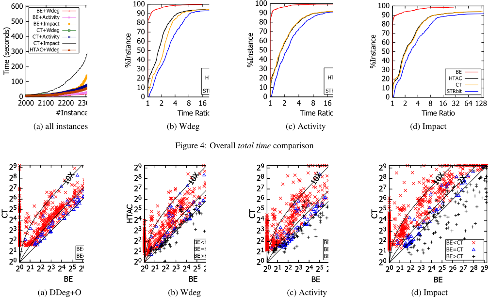
We first evaluate the relative performance of the GAC/AC algorithmic on each variable heuristic. To avoid timeout and small timings, for each variable heuristic, the trivial instances where all algorithms timeout or the solving time of the slowest algorithm is less than 2 seconds are ignored. Thus, different search heuristics have a different number of non-trivial instances. Table 1 gives a relative comparison between BE and other algorithms per search heuristic using total time: 682 instances for Wdeg; 655 for Activity; and 691 for Impact. AvgR is the average ratio of the total time of an algorithm to BE, and MaxR is the maximum total time ratio. The average speedup of BE is between 1.99 to 4.7X and maximum speedup between 19 to 149X. The Initial Time row gives the average initialization time on all 2559 instances, and BE is higher due to the time needed for encoding. #F (fastest) is the number of instances on which an algorithm has the smallest total time. The number of instances on which an algorithm is backtrack free is #BF and timeout is #TO. Overall BE solves more instances than CT, HTAC and STRbit. We highlight that BE is backtrack free on many instances showing that a higher consistency level is effective since GAC has #BF=0 on these instances.
Figure 4a shows the runtime distribution of the total time for all 2559 instances. It shows BE solves more instances than CT/HTAC with Wdeg and better than Impact and Activity, e.g. BE solves 116 more instances than CT with Wdeg for a time limit of 30 seconds/instance. Figure 4b, 4c and 4d show the differences more clearly with performance profiles [Dolan and Mor´e, 2002] comparing the algorithms for each search heuristic on the corresponding non-trivial instances. The yaxis is the percentage of instances and x-axis is the ratio of the CPU time of an algorithm to the virtual best algorithm. BE dominates CT, HTAC and STRbit for all heuristics tested.
Figure 5 gives scatter plots comparing solving times. The solving time of BE is less than that of CT and HTAC on most instances, except instances where BE has the same or more search nodes. A few instances are slower-it turns out that the higher consistency level change the search tree, i.e. filtering impacts the search. To explore this effect, we tested the DDeg/Dom (DDeg) heuristic [Smith and Grant, 1998]. Figure 5a compares BE with CT using the DDeg+O heuristic (for DDeg+O the BE algorithm uses the structure of the original instances to calculate the value of DDeg). With DDeg+O, the number of search nodes of BE is less than or equal to that of CT on all instances tested. The solving time of BE is less than that of CT on all but 10 "BE=CT" instances. For the DDeg heuristic, the solving time of BE is 10X (2X) less than that of CT on 23% (71%) instances. Figures 5b, 5c and 5d give the results of Wdeg, Activity and Impact. For the heuristic Wdeg, Activity and Impact, the solving time of BE is 10X (2X) less than that of HTAC and CT on 27%, 31% and 35% (68%, 69% and 71%) instances, respectively. We see that the Impact heuristic is more affected by consistency levels. We remark that the backtrack free instances with BE can be seen as the points which are on the y-axis.
4, 8}X, Rand-10-20-10, Rand-10-20-60, Rand-15-23-3, Rand-5-1010, Rand-7-40-8t, Rand-8-20-5, Rand-3-20-{20, 20f}.
7 Conclusion
GAC algorithms have been the mainstay of CSP solvers for non-binary CSPs. Recently, the well known hidden variable encoding was shown through the HTAC algorithm to be competitive with state-of-the-art GAC algorithms such as CT on the original non-binary CSP. This is surprising since encoding a non-binary CSP into a binary CSP allowing the use of AC algorithm has been thought to be inferior to GAC on the original non-binary CSP. We show how to further improve the performance of binary encoding with a new binary encoding, the bipartite encoding based on partitioning constraint scopes. Ensuring AC on BE encoded instances not only gives GAC on the original non-binary CSP but may also have higher consistency than GAC. We present an algorithm to construct BE instances with heuristics to keep the representation of the binary constraints compact while encouraging the possibility of higher consistency. We also give a new AC propagator, ACBE, which exploits the structure of BE instances working on connected components of the encoded constraint graph. Extensive experiments comparing solving CSPs with BE versus state-of-the-art GAC algorithms (CT, HTAC and STRbit) on the well known variable search heuristics (Wdeg, Activity, Impact) demonstrate the superiority of solving the CSP with BE. Furthermore, the higher consistency which is achieved also contributes to faster solving and in some cases makes the CSP backtrack free.
Acknowledgments
We acknowledge the support from grant R-726-000-006-646.
@inproceedings{ijcai2020p165,
  title     = {Bipartite Encoding: A New Binary Encoding for Solving Non-Binary CSPs},
  author    = {Wang, Ruiwei and Yap, Roland H.C.},
  booktitle = {Proceedings of the Twenty-Ninth International Joint Conference on
               Artificial Intelligence, {IJCAI-20}},
  publisher = {International Joint Conferences on Artificial Intelligence Organization},
  editor    = {Christian Bessiere},
  pages     = {1184--1191},
  year      = {2020},
  month     = {7},
  note      = {Main track},
  doi       = {10.24963/ijcai.2020/165},
  url       = {https://doi.org/10.24963/ijcai.2020/165},
}
TY - CPAPER TI - Bipartite Encoding: A New Binary Encoding for Solving Non-Binary CSPs AU - Wang, Ruiwei AU - Yap, Roland H.C. T2 - Proceedings of the Twenty-Ninth International Joint Conference on Artificial Intelligence, IJCAI-20 PB - International Joint Conferences on Artificial Intelligence Organization PY - 2020 SP - 1184 EP - 1191 DO - 10.24963/ijcai.2020/165 UR - https://doi.org/10.24963/ijcai.2020/165 ER -Copied
Machine-readable versions of this paper, for tools and AI agents:





