
Semi-Dynamic Hypergraph Neural Network for 3D Pose Estimation
Proceedings of the Twenty-Ninth International Joint Conference on Artificial Intelligence. Main track. Pages 782-788.
https://doi.org/10.24963/ijcai.2020/109
Keywords
- Computer Vision: Biometrics, Face and Gesture Recognition
- Computer Vision: 2D and 3D Computer Vision
- Machine Learning: Deep Learning: Convolutional networks
Abstract
This paper proposes a novel Semi-Dynamic Hypergraph Neural Network (SD-HNN) to estimate 3D human pose from a single image. SD-HNN adopts hypergraph to represent the human body to effectively exploit the kinematic constrains among adjacent and non-adjacent joints. Specifically, a pose hypergraph in SD-HNN has two components. One is a static hypergraph constructed according to the conventional tree body structure. The other is the semi-dynamic hypergraph representing the dynamic kinematic constrains among different joints. These two hypergraphs are combined together to be trained in an end-to-end fashion. Unlike traditional Graph Convolutional Networks (GCNs) that are based on a fixed tree structure, the SD-HNN can deal with ambiguity in human pose estimation. Experimental results demonstrate that the proposed method achieves state-of-the-art performance both on the Human3.6M and MPI-INF-3DHP datasets.
- Method Direct Discuss Eating Greet Phone Photo Pose Purch Sitting SittingD Smoke Wait WalkD Walk WalkT Avg Martinez [Martinez et al., 2017] 51.8 56.2 58.1 59.0 69.5 78.4 55.2 58.1 74.0 94.6 62.3 59.1 65.1 49.5 52.4 62.9 Pavlakos [Pavlakos et al., 2018] 67.4 71.9 66.7 69.1 72.0 77.0 65.0 68.3 83.7 96.5 71.7 65.8 74.9 59.1 63.2 71.9 Fang [Fang et al., 2018] 50.1 54.3 57.0 57.1 66.6 73.3 53.4 55.7 72.8 88.6 60.3 57.7 62.7 47.5 50.6 60.4 Yang [Yang et al., 2018] 51.5 58.9 50.4 57.0 62.1 65.4 49.8 52.7 69.2 85.2 57.4 58.4 43.6 60.1 47.7 58.6 Lee [Lee et al., 2018] 43.8 51.7 48.8 53.1 52.2 74.9 52.7 44.6 56.9 74.3 56.7 66.4 47.5 68.4 45.6 55.8 Trumble [Trumble et al., 2018] 41.7 43.2 52.9 70.0 64.9 83.0 57.3 63.5 61.0 95.0 70.0 62.3 66.2 53.7 52.4 62.5 Chen [Chen et al., 2019] 41.1 44.2 44.9 45.9 46.5 39.3 41.6 54.8 73.2 46.2 48.7 42.1 35.8 46.6 38.5 46.3 Pavllo* [Pavllo et al., 2019] 47.1 50.6 49.0 51.8 53.6 61.4 49.4 47.4 59.3 67.4 52.4 49.5 55.3 39.5 42.7 51.8 Wandt [Wandt and Rosenhahn, 2019] 53.0 58.3 59.6 66.5 72.8 71.0 56.7 69.6 78.3 95.2 66.6 58.5 63.2 57.5 49.9 65.1 Habibie [Habibie et al., 2019] 54.0 65.1 58.5 62.9 67.9 54.0 75.0 60.6 82.7 98.2 63.3 61.2 66.9 50.0 56.5 65.7 Zhao [Zhao et al., 2019] 48.2 60.8 51.8 64.0 64.6 53.6 51.1 67.4 88.7 57.7 73.2 65.6 48.9 64.8 51.9 60.8 Cai* [Cai et al., 2019] 46.5 48.8 47.6 50.9 52.9 61.3 48.3 45.8 59.2 64.4 51.2 48.4 53.5 39.2 41.2 50.6 Ci [Ci et al., 2019] 46.8 52.3 44.7 50.4 52.9 68.9 49.6 46.4 60.2 78.9 51.2 50.0 54.8 40.4 43.3 52.7 SD-HNN 46.5 55.0 54.7 60.2 63.3 48.9 50.2 64.2 54.0 76.0 63.2 55.5 47.6 59.3 44.0 56.2 Martinez [Martinez et al., 2017] (GT) 37.7 44.4 40.3 42.1 48.2 54.9 44.4 42.1 54.6 58.0 45.1 46.4 47.6 36.4 40.4 45.5 Zhao [Zhao et al., 2019](GT) 37.8 49.4 37.6 40.9 45.1 41.4 40.1 48.3 50.1 42.2 53.5 44.3 40.5 47.3 39.0 43.8 SD-HNN (GT) 42.1 45.6 38.2 41.4 41.5 47.4 45.8 39.9 44.7 53.0 42.6 44.0 42.1 34.0 37.6 42.7 Table 1: Quantitative comparisons of Mean Per Joint Position Error (MPJPE) in millimeter between the estimated 3D pose and the ground truth on Human3.6M under Protocol 1. SD-HNN shows the results taking as the input 2D pose estimated by the Stacked Hourglass network. GT means the 2d poses are from the ground truth. The results of Pavllo* and Cai* are based on single frame. Method Direct Discuss Eating Greet Phone Photo Pose Purch Sitting SittingD Smoke Wait WalkD Walk WalkT Avg Martinez [Martinez et al., 2017] 39.5 43.2 46.4 47.0 51.0 56.0 41.4 40.6 56.5 69.4 49.2 45.0 49.5 38.0 43.1 47.7 Lee [Lee et al., 2018] 38.0 39.3 46.3 44.4 49.0 55.1 40.2 41.1 53.2 68.9 51.0 39.1 33.9 56.4 38.5 46.2 Fang [Fang et al., 2018] 38.2 41.7 43.7 44.9 48.5 55.3 40.2 38.2 54.5 64.4 47.2 44.3 47.3 36.7 41.7 45.7 Rayat [Rayat Imtiaz Hossain and Little, 2018] (GT) 35.2 40.8 37.2 37.4 43.2 44.0 38.9 35.6 42.3 44.6 39.7 39.7 40.2 32.8 35.5 39.2 Chen [Chen et al., 2019] 36.5 41.0 40.9 43.9 45.6 53.8 38.5 37.3 53.0 65.2 44.6 40.9 44.3 32.0 38.4 44.1 Wandt [Wandt and Rosenhahn, 2019] (GT) 33.6 38.8 32.6 37.5 36.0 44.1 37.8 34.9 39.2 52.0 37.5 39.8 34.1 40.3 34.9 38.2 SD-HNN 43.7 46.4 39.3 42.7 42.6 48.6 46.6 41.7 45.4 52.5 43.3 45.0 42.4 34.9 38.3 43.5 SD-HNN (GT) 29.6 34.9 31.7 31.6 32.9 37.4 33.3 30.5 37.6 43.0 34.2 34.3 33.2 27.0 29.2 33.4
- [Alex et al., 2012] Krizhevsky Alex, Ilya Sutskever, and Ge- offrey E Hinton. Imagenet classification with deep convo- lutional neural networks. In NeurIPS, pages 1097-1105, 2012.
- [Atwood and Towsley, 2016] James Atwood and Don Towsley. Diffusion-convolutional neural networks. In NeurIPS, pages 1993-2001, 2016.
- [Cai et al., 2019] Yujun Cai, Liuhao Ge, Jun Liu, Jianfei Cai, Tat-Jen Cham, Junsong Yuan, and Nadia Magnenat Thal- mann. Exploiting spatial-temporal relationships for 3d pose estimation via graph convolutional networks. In IC- CV, pages 2272-2281, 2019.
- [Cao et al., 2017] Zhe Cao, Tomas Simon, Shih En Wei, and Yaser Sheikh. Realtime multi-person 2d pose estimation using part affinity fields. In CVPR, pages 1302-1310, 2017.
- [Chen and Ramanan, 2017] Ching-Hang Chen and Deva Ra- manan. 3d human pose estimation= 2d pose estimation+ matching. In CVPR, pages 5759-5767. IEEE, 2017.
- [Chen et al., 2019] Xipeng Chen, Kwan-Yee Lin, Wentao Liu, Chen Qian, and Liang Lin. Weakly-supervised dis- covery of geometry-aware representation for 3d human pose estimation. In CVPR, pages 10895-10904, 2019.
- [Chu et al., 2017] Xiao Chu, Wei Yang, Wanli Ouyang, Cheng Ma, Alan L Yuille, and Xiaogang Wang. Multi- context attention for human pose estimation. In CVPR, pages 1831-1840, 2017.
- [Ci et al., 2019] Hai Ci, Chunyu Wang, Xiaoxuan Ma, and Yizhou Wang. Optimizing network structure for 3d human pose estimation. In CVPR, pages 2262-2271, 2019.
- [Fang et al., 2018] Haoshu Fang, Yuanlu Xu, Wenguan Wang, Xiaobai Liu, and Song-Chun Zhu. Learning knowledge-guided pose grammar machine for 3d human pose estimation. In AAAI, 2018.
- [Feng et al., 2019] Yifan Feng, Haoxuan You, Zizhao Zhang, Rongrong Ji, and Yue Gao. Hypergraph neural net- works. In AAAI, volume 33, pages 3558-3565, 2019.
- [Habibie et al., 2019] Ikhsanul Habibie, Weipeng Xu, Dushyant Mehta, Gerard Pons-Moll, and Christian Theobalt. In the wild human pose estimation using explicit 2d features and intermediate 3d representations. In CVPR, June 2019.
- [Insafutdinov et al., 2016] Eldar Insafutdinov, Leonid Pishchulin, Bjoern Andres, Mykhaylo Andriluka, and Bernt Schiele. Deepercut: A deeper, stronger, and faster multi-person pose estimation model. In ECCV, pages 34-50. Springer, 2016.
- [Kipf and Welling, 2016] Thomas N Kipf and Max Welling. Semi-supervised classification with graph convolutional networks. arXiv preprint arXiv:1609.02907, 2016.
- [Lee et al., 2018] Kyoungoh Lee, Inwoong Lee, and Sanghoon Lee. Propagating lstm: 3d pose estimation based on joint interdependency. In ECCV, pages 119-135, 2018.
- [Martinez et al., 2017] Julieta Martinez, Rayat Hossain, Javier Romero, and James J Little. A simple yet effective baseline for 3d human pose estimation. In ICCV, pages 2640-2649, 2017.
- [Michel et al., 2015] Frank Michel, Alexander Krull, Eric Brachmann, Michael Ying Yang, Stefan Gumhold, and Carsten Rother. Pose estimation of kinematic chain in- stances via object coordinate regression. In BMVC, 2015.
- [Moreno-Noguer, 2017] Francesc Moreno-Noguer. 3d hu- man pose estimation from a single image via distance ma- trix regression. In CVPR, pages 1561-1570, 2017.
- [Newell et al., 2016] Alejandro Newell, Kaiyu Yang, and Jia Deng. Stacked hourglass networks for human pose esti- mation. In ECCV, pages 483-499. Springer, 2016.
- [Pavlakos et al., 2017] Georgios Pavlakos, Xiaowei Zhou, Konstantinos G. Derpanis, and Kostas Daniilidis. Coarse- to-fine volumetric prediction for single-image 3d human pose. In CVPR, pages 1263-1272, 2017.
- [Pavlakos et al., 2018] Georgios Pavlakos, Xiaowei Zhou, and Kostas Daniilidis. Ordinal depth supervision for 3d human pose estimation. In CVPR, pages 7307-7316, 2018.
- [Pavllo et al., 2019] Dario Pavllo, Christoph Feichtenhofer, David Grangier, and Michael Auli. 3d human pose es- timation in video with temporal convolutions and semi- supervised training. In CVPR, June 2019.
- [Rayat Imtiaz Hossain and Little, 2018] Mir Rayat Imti- az Hossain and James J Little. Exploiting temporal information for 3d human pose estimation. In ECCV, pages 68-84, 2018.
- [Sun et al., 2018] Xiao Sun, Bin Xiao, Fangyin Wei, Shuang Liang, and Yichen Wei. Integral human pose regression. In ECCV, September 2018.
- [Trumble et al., 2018] Matthew Trumble, Andrew Gilbert, Adrian Hilton, and John Collomosse. Deep autoencoder for combined human pose estimation and body model up- scaling. In ECCV, pages 784-800, 2018.
- [Wandt and Rosenhahn, 2019] Bastian Wandt and Bodo Rosenhahn. Repnet: Weakly supervised training of an ad- versarial reprojection network for 3d human pose estima- tion. In CVPR, pages 7782-7791, 2019.
- [Yan et al., 2018] Sijie Yan, Yuanjun Xiong, and Dahua Lin. Spatial temporal graph convolutional networks for skeleton-based action recognition. In AAAI, 2018.
- [Yang et al., 2018] Wei Yang, Wanli Ouyang, Xiaolong Wang, Jimmy Ren, Hongsheng Li, and Xiaogang Wang. 3d human pose estimation in the wild by adversarial learn- ing. In CVPR, pages 5255-5264, 2018.
- [Zhao et al., 2019] Long Zhao, Xi Peng, Yu Tian, Mubbasir Kapadia, and Dimitris N Metaxas. Semantic graph convo- lutional networks for 3d human pose regression. In CVPR, pages 3425-3435, 2019.
- [Zhou et al., 2017] Xingyi Zhou, Qixing Huang, Xiao Sun, Xiangyang Xue, and Yichen Wei. Towards 3d human pose estimation in the wild: a weakly-supervised approach. In CVPR, pages 398-407, 2017.
References were extracted automatically from the PDF and may contain errors.
Full text extracted automatically from the PDF; figures, tables and equations may differ. The PDF is the version of record.
1 Introduction
Pose estimation aims to estimate 2D or 3D positions of human body joints from an image or video. It is an active research area in computer vision due to its wide range of potential applications. Like many other areas in computer vision, Convolutional Neural Networks (CNN) [Alex et al., 2012] have also been used for pose estimation. There are generally two kinds of CNN-based approaches. One is to directly estimate 3D human pose through a CNN [Sun et al., 2018] from an image. The other is to estimate a 2D pose through a CNN first, and then recover the 3D pose from the estimated 2D pose [Martinez et al., 2017; Moreno-Noguer, 2017; Pavlakos et al., 2017; Rayat Imtiaz Hossain and Little, 2018]. The former approach usually requires sufficient amount of annotated data and much computing resource for training where the latter may not utilize visual information in the second stage for 3D recovery. However, the human body is a typical chain-like structure constrained by human kinematics. Most of CNN-based pose estimation do not leverage this prior information.
∗Corresponding author
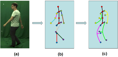
Graph Convolutional Network (GCNs) [Kipf andWelling, 2016] as a generalization of CNNs to deal with non-Euclidean data can learn feature representation of a graph through gradually aggregating features of multiple nodes to compute features for a node of interest. Some attempts of using GCN for 3D pose estimation are reported in [Yan et al., 2018; Zhao et al., 2019; Cai et al., 2019; Ci et al., 2019]. Although these methods have achieved promising results, they are limited by the fact that they all treat the human body as a tree structure and represent it as a simplified graph. According to human kinematics, the human body has a typical chainlike structure. The movement of body joints is not only constrained by directly neighboring joints, but also is subject to multiple non-neighboring joints. Such a complex relationship can hardly be captured by a simple graph with a set of fixed connections between joints.
To address this problem, we propose to represent the hu[Feng et al., 2019] aiming to learn local and global kinematic constrains among joints (shown in Figure 1). Unlike a simple graph, a hypergraph represents the human body and its kinematic constrains with flexible hyperedges. These hyperedges have no fixed degrees and are able to connect different body joints freely according to the dy-
namic interaction relationships among them. This characteristic conforms to the concept of the kinematic chain [Michel et al., 2015] and is able to model the kinematic constrains through adding or deleting hyperedge dynamically.
Upon the hypergraph representation of the human body, this paper develops a novel semi-dynamic hypergraph neural network (SD-HNN) for 3D human pose estimation. Specifically, based on the knowledge of human kinematic chain, we treat a series of closely related joints as a whole to construct a static hypergraph, and each kinematic chain will be regarded as a hyperedge in the hypergraph. In addition, we also construct a dynamic hypergraph of a human body, whose structure will be changed in the course of convolution operation along with the convolution kernel. The motivation is inspired that the kinematic constrains or the effects among different body joints may be different under different poses. A dynamic hypergraph is able to deal with the above situation intuitively. The static and dynamic hypergraphs are combined together and trained in an end-to-end fashion. We refer to such a scheme as being semi-dynamic.
Overall, the key contributions of this paper are:
- We propose to represent a human body as a hypergraph and, hence, to capture human kinematics using a combination of a static hypergraph and a dynamic hypergraph.
- Upon the representation, we develop a semi-dynamic hypergraph neural network (SD-HNN) for recovering 3D poses from 2D poses, which can be trained in an end-to-end way.
- The proposed representation and SD-HNN are extensively validated on Human 3.6m and MPI-INF-3DHP datasets. Their effectiveness has been demonstrated by the state-of-the-art performance.
2 RelatedWork
In the past few years, hand-crafted features, such as HOG, SIFT, DPM, are commonly used for 3D human pose regression. Recently, many state-of-the-art methods are based on deep convolution neural networks to estimate 3D human pose. As 2D human pose estimation [Cao et al., 2017; Chu et al., 2017; Insafutdinov et al., 2016] advances, a twostage framework becomes popular for 3D human pose estimation. In this framework, the 2D human pose is estimated or predicted in the first stage by a CNN, and then the 2D pose together with the intermediate layer features from the CNN are used to regress 3D pose [Chen and Ramanan, 2017; Martinez et al., 2017; Pavlakos et al., 2017; Fang et al., 2018]. The proposed SD-HNN follows the two-stage framework.
Graph Neural Networks (GNNs) have also been used in pose estimation. Construction of GCNs on a graph generally follows either spatial perspective or spectral perspective. Convolution operations directly on the graph are implemented in [Atwood and Towsley, 2016; Ci et al., 2019; Cai et al., 2019], while in [Kipf and Welling, 2016] convolution operations are in the spectral domain. Specifically, ST-GCN [Yan et al., 2018] and SEM-GCN [Zhao et al., 2019] both follow the spatial perspective. ST-GCN is probably the first representative work to adopt graph-based neural networks to model dynamic skeletons for action recognition. SEM-GCN employed GCNs to regress 3D pose from 2D by capturing both local and global relationships among joints. This paper extends GCN to a hypergraph neural network (HNN) in order to better capture human kinematics.
3 Semi-Dynamic Hypergraph Neural Network
In this section, we first briefly introduce GCN and the concept of HNN. With these preliminary knowledge, details of the proposed Semi-Dynamic Hypergraph following together with the network structure based on it will be demonstrated.
3.1 GCN and HNN
Assume that an input graph is G= {A,X}. The adjacency matrix is A ∈ Rn×n . Specifically, A = [aij] ∈ Rn×n gives the connectivity information between different nodes, while aij > 0 means there exists an edge between node i and node j. The node set is X ∈ Rn×d , which is treated as input signal on the graph. n represents the number of vertex on graph, d is the dimension of feature. Based on above terminologies, a standard convolution of GCN [Kipf and Welling, 2016] can be represented as follows:
where H(l) denotes the representation of graph nodes in the l-th layer, W (l) stands for the model parameters in the l-th layer, σ (·) represents a non-linear activation function. Additionally, ∼A represents a normalized graph adjacency matrix. Here, ∼A = A+ I, where I is the degree matrix of the image.
The concept of GCN is extended to hypergraph in [Feng et al., 2019] and a new hypergraph neural network (HNN) framework is proposed. The convolution of HNN is reformulated as follows:
where Dv, De denote the diagonal matrices of the vertex degrees and the edge degrees respectively. The filter Γ is applied over the nodes in hypergraph to extract features.
3.2 Semi-Dynamic Hypergraph
In previous work, the human body is often represented as a tree structure. There are 5 common pieces of pre-defined kinematic chains, where 4 pieces represent the limbs respectively and 1 represents the body trunk. In such fixed structural representation, the connections among different joints only represent physical relationships, which cannot cover those potential non-physical connections among other joints while the human is moving. Therefore, we involve the novel hypergraph to describe the kinematic characteristics of human body and construct a semi-dynamic HNN model to address above shortcoming.
Compared with simple graph, each edge in hypergraph can connect more than two nodes. First of all, we transform previous common pieces of pre-defined kinematic chains into 5 hyperedges, each hyperedge corresponding to the kinematic chain connects all of the joints in that kinematic chain. We call this representation as static hypergraph, since it will be used as the fundamental structure for all the human poses. However, there may be some potential connections among different non-adjacent joints under kinematic constrains, which are ignored directly by such hypergraph structure.
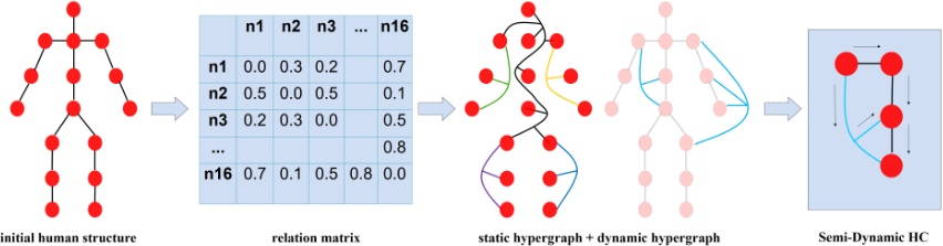
To solve this problem, we try to connect those joints which may have potential relation under kinematic constrains into same hyperedges in our hypergraph dynamically. For example, in movement category 'sitting', the hyperedges in our hypergraph may contain more joints from legs, which is different from the movement category such as 'greeting'. Finally, We introduce a new semi-dynamic hypergraph (Figure 2), which contains 5 common pre-defined static hyperedges and different numbers of dynamic hyperedges, as our hypergraph represention of human body.
Before explaining the convolution process on dynamic hypergraph, we introduce how to construct this kind of hypergraph. First, we define a set of hyperedges S, and then construct the hypergraph only by the hyperedges in S. The S contains two parameters, Emax represents the number of edges in dynamic hypergraph, Mmax represents the maxium number of nodes in one hyperedge. We add joint i and joint j into one hyperedge according to their distance. Inspired by some previous work, the relation between two nodes in hyperedge can be calculated according to the formula below:
where Dist is the distance between two joints in feature space, and the Θ is a weight factor matrix. When two joints i and j are very close in graph, the Θ(i, j) will be a small value, while i and j are very far from each other, the Θ(i, j) will be larger. Since the dynamic hypergraph is designed for capturing the relationship between non-adjacent joints and overcome the limitations of traditional tree structure, different joints will have more chance to be connected together. Through setting different Emax and Mmax values, various dynamic hypergraphs can be constructed as our input. In our experiment, the optimal number of hyperedges and that of nodes in a hyperedge can be seen in the ablation study part. The details can be referred to Algorithm 1.
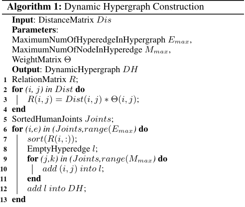
We follow the method in [Feng et al., 2019] for hypergraph convolutions. Different from graph convolution, the hypergraph convolution is a node-edge-node transform. For the input feature X ∈ RN×C , by left multiplying HT ∈ RE×N , we can estimate the edge feature of RE×C , where H is the hyperedge incidence matrix. The edge-node transform is quite same but the order of multiplication is opposite. Since we already know the H in our hypergraph, the node-edge-node transform can be reduced to node-node transform.
Compared with the 'vanilla' HNN, the main difference is that our model involves two types of hypergraph convolutions, the fixed ones and dynamic ones, to enforce the kinematic constrains of human body as illustrated in Figure 2. The convolution on static hypergraph is quite similar to the 'vanilla' HNN. Let Xl be the output of l-th hypergraph layer, and σ denotes a nonlinear activation function. W represents a learnable weight matrix of l-th hypergraph layer and Hs represents the kernel for node-node transform which can be calculated from the input hypergraph structure. The static graph convolution can be expressed as:
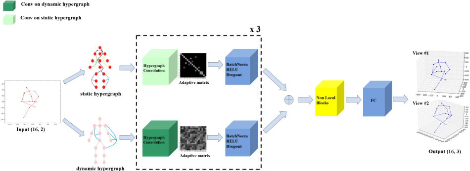
To deal with different dynamic hypergraph structures, we add an adaptive weighting matrix M in SD-HNN. Combining the static part and the dynamic part together, we get a complete formula of our network convolution in Equation 5:
where F (l) is the output of l-th hypergraph layer, D is convolution kernel of dynamic hypergraph and M is an adaptive weighting matrix which can be learned during training. In summary, the information propagation in our method is a combination of static part and dynamic part, which is one kind of semi-dynamic way. For each part, the model will perform the convolution independently, exploring the information between neighborhood and global joints, and then weighting matrix will be updated iteratively.
Compared with other GCN models, we have the following two obvious differences: (1) The hypergraph is first involved in our model to estimate the 3D human pose, which is able to better formulate the complex kinematic relationship among human joints. (2) Our network can deal with different hypergraphs, and the corresponding learnable matrix are used to adapt to the dynamic changes of these hypergraph structures. These two characteristics make our network more robust for 3D pose estimation.
3.3 Framework Overview
Figure 3 shows the proposed SD-HNN, which takes a series of 2D poses as input. The input is formally defined as (ν, e), which includes a 2D joints set ν, and a hyperedge based skeleton set e. Suppose P is a set with N 2D joints, and their corresponding 3D joints under predefined camera coordinate system is J, our method aims to learn a regression function A
to minimizes the following error on a dataset of human poses that contains N samples:
where Iproj is the inverse transformation of projection and L computes the L2 distance. This regression function can be trained in an end-to-end fasion.
4 Experiments
4.1 Implementation Details
In our experiment, the Stacked Hourglass network [Newell et al., 2016] is adopted as the basic 2D pose detector and is initialized with weights pre-trained on the MPII dataset and fineturned on Human3.6M. Our model is trained with Adam optimizer for 100 epochs, learning rate of 0.001 and batch size of 256. ReLU is chosen as the nonlinear activation function. The hidden dimension of our method is 256, which means the input data with the shape of (16,2) is mapped into a 256 dimension vector.
4.2 Datasets And Protocols
We evaluate the proposed method on two datasets: Human3.6M and MPI-INF-3DHP. The Human3.6M is one of the largest datasets for 3D human pose estimation. It consists of 3.6 millions of images featuring 11 actors performing 15 daily activities, such as walking, eating, sitting and smoking with 4 camera views. Simultaneously, the dataset also provides some important basic data such as camera parameters, ground truth data of 2D and 3D pose. We use the subject 1, 5, 6, 7 and 8 in Human3.6m for training and subject 9 and 11 for testing. Similar to most of single-frame human pose estimation methods, our method down-sample the data of Human3.6m, and for the video data from original 50fps to 10fps.
| Method | Direct | Discuss | Eating | Greet | Phone | Photo | Pose | Purch | Sitting | SittingD | Smoke | Wait | WalkD | Walk | WalkT | Avg |
|---|---|---|---|---|---|---|---|---|---|---|---|---|---|---|---|---|
| Martinez [Martinez et al., 2017] | 51.8 | 56.2 | 58.1 | 59.0 | 69.5 | 78.4 | 55.2 | 58.1 | 74.0 | 94.6 | 62.3 | 59.1 | 65.1 | 49.5 | 52.4 | 62.9 |
| Pavlakos [Pavlakos et al., 2018] | 67.4 | 71.9 | 66.7 | 69.1 | 72.0 | 77.0 | 65.0 | 68.3 | 83.7 | 96.5 | 71.7 | 65.8 | 74.9 | 59.1 | 63.2 | 71.9 |
| Fang [Fang et al., 2018] | 50.1 | 54.3 | 57.0 | 57.1 | 66.6 | 73.3 | 53.4 | 55.7 | 72.8 | 88.6 | 60.3 | 57.7 | 62.7 | 47.5 | 50.6 | 60.4 |
| Yang [Yang et al., 2018] | 51.5 | 58.9 | 50.4 | 57.0 | 62.1 | 65.4 | 49.8 | 52.7 | 69.2 | 85.2 | 57.4 | 58.4 | 43.6 | 60.1 | 47.7 | 58.6 |
| Lee [Lee et al., 2018] | 43.8 | 51.7 | 48.8 | 53.1 | 52.2 | 74.9 | 52.7 | 44.6 | 56.9 | 74.3 | 56.7 | 66.4 | 47.5 | 68.4 | 45.6 | 55.8 |
| Trumble [Trumble et al., 2018] | 41.7 | 43.2 | 52.9 | 70.0 | 64.9 | 83.0 | 57.3 | 63.5 | 61.0 | 95.0 | 70.0 | 62.3 | 66.2 | 53.7 | 52.4 | 62.5 |
| Chen [Chen et al., 2019] | 41.1 | 44.2 | 44.9 | 45.9 | 46.5 | 39.3 | 41.6 | 54.8 | 73.2 | 46.2 | 48.7 | 42.1 | 35.8 | 46.6 | 38.5 | 46.3 |
| Pavllo* [Pavllo et al., 2019] | 47.1 | 50.6 | 49.0 | 51.8 | 53.6 | 61.4 | 49.4 | 47.4 | 59.3 | 67.4 | 52.4 | 49.5 | 55.3 | 39.5 | 42.7 | 51.8 |
| Wandt [Wandt and Rosenhahn, 2019] | 53.0 | 58.3 | 59.6 | 66.5 | 72.8 | 71.0 | 56.7 | 69.6 | 78.3 | 95.2 | 66.6 | 58.5 | 63.2 | 57.5 | 49.9 | 65.1 |
| Habibie [Habibie et al., 2019] | 54.0 | 65.1 | 58.5 | 62.9 | 67.9 | 54.0 | 75.0 | 60.6 | 82.7 | 98.2 | 63.3 | 61.2 | 66.9 | 50.0 | 56.5 | 65.7 |
| Zhao [Zhao et al., 2019] | 48.2 | 60.8 | 51.8 | 64.0 | 64.6 | 53.6 | 51.1 | 67.4 | 88.7 | 57.7 | 73.2 | 65.6 | 48.9 | 64.8 | 51.9 | 60.8 |
| Cai* [Cai et al., 2019] | 46.5 | 48.8 | 47.6 | 50.9 | 52.9 | 61.3 | 48.3 | 45.8 | 59.2 | 64.4 | 51.2 | 48.4 | 53.5 | 39.2 | 41.2 | 50.6 |
| Ci [Ci et al., 2019] | 46.8 | 52.3 | 44.7 | 50.4 | 52.9 | 68.9 | 49.6 | 46.4 | 60.2 | 78.9 | 51.2 | 50.0 | 54.8 | 40.4 | 43.3 | 52.7 |
| SD-HNN | 46.5 | 55.0 | 54.7 | 60.2 | 63.3 | 48.9 | 50.2 | 64.2 | 54.0 | 76.0 | 63.2 | 55.5 | 47.6 | 59.3 | 44.0 | 56.2 |
| Martinez [Martinez et al., 2017] (GT) | 37.7 | 44.4 | 40.3 | 42.1 | 48.2 | 54.9 | 44.4 | 42.1 | 54.6 | 58.0 | 45.1 | 46.4 | 47.6 | 36.4 | 40.4 | 45.5 |
| Zhao [Zhao et al., 2019](GT) | 37.8 | 49.4 | 37.6 | 40.9 | 45.1 | 41.4 | 40.1 | 48.3 | 50.1 | 42.2 | 53.5 | 44.3 | 40.5 | 47.3 | 39.0 | 43.8 |
| SD-HNN (GT) | 42.1 | 45.6 | 38.2 | 41.4 | 41.5 | 47.4 | 45.8 | 39.9 | 44.7 | 53.0 | 42.6 | 44.0 | 42.1 | 34.0 | 37.6 | 42.7 |
| Method | Direct | Discuss | Eating | Greet | Phone | Photo | Pose | Purch | Sitting | SittingD | Smoke | Wait | WalkD | Walk | WalkT | Avg |
|---|---|---|---|---|---|---|---|---|---|---|---|---|---|---|---|---|
| Martinez [Martinez et al., 2017] | 39.5 | 43.2 | 46.4 | 47.0 | 51.0 | 56.0 | 41.4 | 40.6 | 56.5 | 69.4 | 49.2 | 45.0 | 49.5 | 38.0 | 43.1 | 47.7 |
| Lee [Lee et al., 2018] | 38.0 | 39.3 | 46.3 | 44.4 | 49.0 | 55.1 | 40.2 | 41.1 | 53.2 | 68.9 | 51.0 | 39.1 | 33.9 | 56.4 | 38.5 | 46.2 |
| Fang [Fang et al., 2018] | 38.2 | 41.7 | 43.7 | 44.9 | 48.5 | 55.3 | 40.2 | 38.2 | 54.5 | 64.4 | 47.2 | 44.3 | 47.3 | 36.7 | 41.7 | 45.7 |
| Rayat [Rayat Imtiaz Hossain and Little, 2018] (GT) | 35.2 | 40.8 | 37.2 | 37.4 | 43.2 | 44.0 | 38.9 | 35.6 | 42.3 | 44.6 | 39.7 | 39.7 | 40.2 | 32.8 | 35.5 | 39.2 |
| Chen [Chen et al., 2019] | 36.5 | 41.0 | 40.9 | 43.9 | 45.6 | 53.8 | 38.5 | 37.3 | 53.0 | 65.2 | 44.6 | 40.9 | 44.3 | 32.0 | 38.4 | 44.1 |
| Wandt [Wandt and Rosenhahn, 2019] (GT) | 33.6 | 38.8 | 32.6 | 37.5 | 36.0 | 44.1 | 37.8 | 34.9 | 39.2 | 52.0 | 37.5 | 39.8 | 34.1 | 40.3 | 34.9 | 38.2 |
| SD-HNN | 43.7 | 46.4 | 39.3 | 42.7 | 42.6 | 48.6 | 46.6 | 41.7 | 45.4 | 52.5 | 43.3 | 45.0 | 42.4 | 34.9 | 38.3 | 43.5 |
| SD-HNN (GT) | 29.6 | 34.9 | 31.7 | 31.6 | 32.9 | 37.4 | 33.3 | 30.5 | 37.6 | 43.0 | 34.2 | 34.3 | 33.2 | 27.0 | 29.2 | 33.4 |
The Mean Per Joint Position Error (MPJPE) is used to measure the error between the results and ground truth, that is, ground truth and estimated value are aligned to the root point and then are used to calculate the error. We call this process as Protocol 1. Besides, there are some other work calculating P-MPJPE at the same time, that is, the ground truth and the estimated pose are both aligned through rigid transformation. We call the process as Protocol 2.
MPI-INF-3DHP is a 3D human pose dataset using MoCap system. The test set contains 2929 valid frames from 6 subjects, performing 7 actions. We employ average PCK (with a threshold 150mm) and AUC as the evaluation metrics.
4.3 Quantitative Results
Human3.6M Dataset. We take the 2D pose detected by the Stacked Hourglass network(SH) and the ground truth 2D pose of Human3.6m as the input respectively. Table 1 shows the quantitative comparisons of MPJPE between the estimated pose and the ground-truth on Human3.6M under Protocol 1. As shown in this table, our method achieves competitive results with inaccurate 2D poses, and outperforms other stateof-the-art methods on most individual actions and the best average accuracy with ground truth 2D data. Table 2 shows the quantitative comparisons of MPJPE under Protocol 2. With the ground truth 2D pose as the input, our method achieves the best results.
MPI-INF-3DHP Dataset. Table 3 shows the comparison results between our proposed method with other state-of-theart methods on the MPI-INF-3DHP dataset. We train our model only with Human3.6M data. Our proposed method achieves the best result, since the semi-dynamic hypergraph and its corresponding convolution operation can enforce more kinematic constrains to enhance the generalization capability of our model.
| Method | Training Data | PCK | AUC |
|---|---|---|---|
| Zhou [Zhou et al., 2017] | H3.6m+MPII | 69.2 | 32.5 |
| Yang [Yang et al., 2018] | H3.6m+MPII | 69.0 | 32.0 |
| Pavlakos* [Pavlakos et al., 2018] | H3.6m+MPII+LSP | 71.9 | 35.3 |
| Habibie [Habibie et al., 2019] | H3.6m | 70.4 | 36.0 |
| Ci [Ci et al., 2019] | H3.6m | 74.0 | 36.7 |
| SD-HNN | H3.6m | 74.9 | 37.5 |
4.4 Ablation Study
In this section, we will verify the effectiveness of different dynamic components in our method on the Human3.6M dataset under Protocol 1. For the effect of initial hypergraph structure on final results, different numbers of hyperedge are set in our initial hypergraph and the results are shown in Table 4. From this table, we can see that when the number of hyperedges is changed from 5 to 20, the results almost keep the same, which means that the ability of our proposed method in constructing dynamic hypergraphs does not depend on the input heavily. Even only 5 pieces of hyperedges are contained in the hypergrah, which only contains the static part, our SD- HNN still can well represent the human body along with its kinematic characteristics by leveraging the corresponding semi-dynamic hypergraph.
| Number of hyperedges | MPJPE(GT) |
|---|---|
| 5 | 43.8 |
| 7 | 42.7 |
| 10 | 43.4 |
| 20 | 43.9 |
| Method | MPJPE (GT) |
|---|---|
| w/o dynamic graph | 43.8 |
| with dynamic graph | 42.7 |
To prove the role of semi-dynamic hypergraph in our proposed method, we test SD-HNN on Human3.6M test data with or without dynamic hypergraphs. Table 5 shows the result and demonstrates the dynamic hypergraph part really has improved the performance of HNN by establishing more reasonable connections.
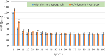
Figure 4 shows the changes of MPJPE in network training with or without dynamic hypergraph. From this table, we can see the introduction of dynamic hypergraph into SD-HNN accelerates the convergence speed during early stage of training, and also achieves better results eventually.
4.5 Qualitative Study
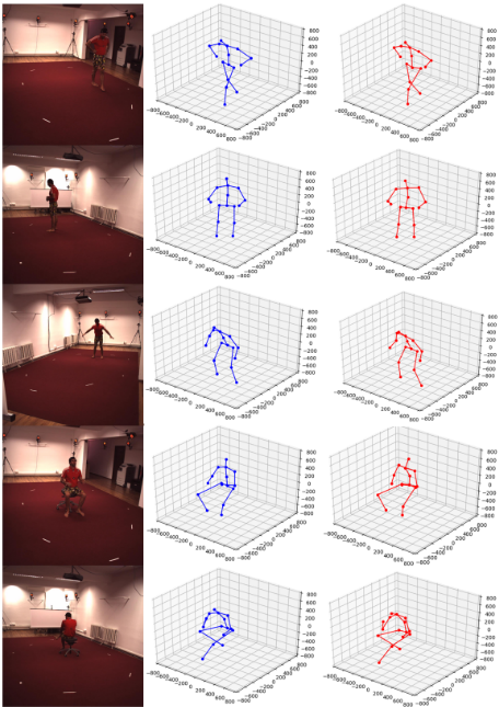
Some results on the Human3.6M are visuzlided in Figure 5. In this figure, the estimated 3D poses with ground truth are compared. From the results, we can see even the human perform complex actions or have self-occlusion, the proposed method still can generate right results.
5 Conclusion
In this paper, we propose a novel Semi-Dynamic Hypergraph Neural Network (SD-HNN) to estimate 3D human pose. SDHNN adopts hypergraph to represent human body to effectively exploit the kiematic constrains among adjacent and non-adjacent joints. A pose hypergraph in SD-HNN has a static component constructed according to the conventional tree body structure, and a dynamic component representing the dynamic kinematic constrains among different joints. These two hypergraphs are combined together to be trained in an end-to-end way. Unlike traditional Graph Convolutional Networks (GCNs) that are based on a fixed tree structure, the SD-HNN is able to deal with ambiguity in human pose estimation. The proposed method achieves state-of-the-art performance on both Human3.6M and MPI-INF-3DHP datasets. In the future, we will further explore other efficient methods to make better use of edge features in hypergraph for more challenge works, such as multiple person pose estimation.
Acknowledgments
The authors would like to thank all the anonymous reviewers. This work was supported by National Natural Science Foundation of China under Grant Number 61772474, 61822701, 61872324, Program for Science & Technology Innovation Talents in Universities of Henan Province(20HASTIT021) and Youth Talent Promotion Project in Henan Province (2019HYTP022).
@inproceedings{ijcai2020p109,
  title     = {Semi-Dynamic Hypergraph Neural Network for 3D Pose Estimation},
  author    = {Liu, Shengyuan and Lv, Pei and Zhang, Yuzhen and Fu, Jie and Cheng, Junjin and Li, Wanqing and Zhou, Bing and Xu, Mingliang},
  booktitle = {Proceedings of the Twenty-Ninth International Joint Conference on
               Artificial Intelligence, {IJCAI-20}},
  publisher = {International Joint Conferences on Artificial Intelligence Organization},
  editor    = {Christian Bessiere},
  pages     = {782--788},
  year      = {2020},
  month     = {7},
  note      = {Main track},
  doi       = {10.24963/ijcai.2020/109},
  url       = {https://doi.org/10.24963/ijcai.2020/109},
}
TY - CPAPER TI - Semi-Dynamic Hypergraph Neural Network for 3D Pose Estimation AU - Liu, Shengyuan AU - Lv, Pei AU - Zhang, Yuzhen AU - Fu, Jie AU - Cheng, Junjin AU - Li, Wanqing AU - Zhou, Bing AU - Xu, Mingliang T2 - Proceedings of the Twenty-Ninth International Joint Conference on Artificial Intelligence, IJCAI-20 PB - International Joint Conferences on Artificial Intelligence Organization PY - 2020 SP - 782 EP - 788 DO - 10.24963/ijcai.2020/109 UR - https://doi.org/10.24963/ijcai.2020/109 ER -Copied
Machine-readable versions of this paper, for tools and AI agents:





