
mdfa: Multi-Differential Fairness Auditor for Black Box Classifiers
Proceedings of the Twenty-Eighth International Joint Conference on Artificial Intelligence. AI for Improving Human Well-being. Pages 5871-5879.
https://doi.org/10.24963/ijcai.2019/814
Keywords
- Special Track on AI for Improving Human-Well Being: AI ethics (Special Track on AI and Human Wellbeing)
- Special Track on AI for Improving Human-Well Being: Societal applications (Special Track on AI and Human Wellbeing)
- Special Track on AI for Improving Human-Well Being: Well being metrics (Special Track on AI and Human Wellbeing)
Abstract
Machine learning algorithms are increasingly involved in sensitive decision-making processes with adversarial implications on individuals. This paper presents a new tool, mdfa that identifies the characteristics of the victims of a classifier's discrimination. We measure discrimination as a violation of multi-differential fairness. Multi-differential fairness is a guarantee that a black box classifier's outcomes do not leak information on the sensitive attributes of a small group of individuals. We reduce the problem of identifying worst-case violations to matching distributions and predicting where sensitive attributes and classifier's outcomes coincide. We apply mdfa to a recidivism risk assessment classifier widely used in the United States and demonstrate that for individuals with little criminal history, identified African-Americans are three-times more likely to be considered at high risk of violent recidivism than similar non-African-Americans.
- [Agarwal et al., 2018] Alekh Agarwal, Alina Beygelzimer, Miroslav Dudík, John Langford, and Hanna Wallach. A reductions approach to fair classification. arXiv preprint arXiv:1803.02453, 2018.
- [Atlantic, 2016] The Atlantic. How algorithms can bring down minorities credit scores? The Atlantic, 2016. https://www.theatlantic.com/technology/archive/2016/12/ how-algorithms-can-bring-down-minorities-credit-scores/ 509333/. Link
- [Calsamiglia, 2009] Caterina Calsamiglia. Decentralizing equality of opportunity. International Economic Review, 50(1):273-290, 2009.
- [Chouldechova and Roth, 2018] Alexandra Chouldechova and Aaron Roth. The frontiers of fairness in machine learning. arXiv preprint arXiv:1810.08810, 2018.
- [Cortes et al., 2008] Corinna Cortes, Mehryar Mohri, Michael Riley, and Afshin Rostamizadeh. Sample selec- tion bias correction theory. In International Conference on Algorithmic Learning Theory, pages 38-53. Springer, 2008.
- [Cortes et al., 2010] Corinna Cortes, Yishay Mansour, and Mehryar Mohri. Learning bounds for importance weight- ing. In Advances in neural information processing sys- tems, pages 442-450, 2010.
- [Dwork et al., 2012] Cynthia Dwork, Moritz Hardt, Toniann Pitassi, Omer Reingold, and Richard Zemel. Fairness through awareness. In Proceedings of the 3rd innovations in theoretical computer science conference, pages 214- 226. ACM, 2012.
- [Dwork et al., 2014] Cynthia Dwork, Aaron Roth, et al. The algorithmic foundations of differential privacy. Founda- tions and Trends R in Theoretical Computer Science, 9(3- 4):211-407, 2014.
- [Feldman et al., 2012] Vitaly Feldman, Venkatesan Gu- ruswami, Prasad Raghavendra, and Yi Wu. Agnostic learn- ing of monomials by halfspaces is hard. SIAM Journal on Computing, 41(6):1558-1590, 2012.
- [Feldman et al., 2015] Michael Feldman, Sorelle A Friedler, John Moeller, Carlos Scheidegger, and Suresh Venkata- subramanian. Certifying and removing disparate impact. In Proceedings of the 21th ACM SIGKDD International Conference on Knowledge Discovery and Data Mining, pages 259-268. ACM, 2015.
- [Foulds and Pan, 2018] James Foulds and Shimei Pan. An intersectional definition of fairness. arXiv preprint arXiv:1807.08362, 2018.
- [Friedler et al., 2018] Sorelle A Friedler, Carlos Scheideg- ger, Suresh Venkatasubramanian, Sonam Choudhary, Evan P Hamilton, and Derek Roth. A comparative study of fairness-enhancing interventions in machine learning. arXiv preprint arXiv:1802.04422, 2018.
- [Gretton et al., 2009] Arthur Gretton, Alex J Smola, Jiayuan Huang, Marcel Schmittfull, Karsten M Borgwardt, and Bernhard Schöllkopf. Covariate shift by kernel mean matching. In Dataset shift in machine learning, pages 131-160. MIT Press, 2009.
- [Hébert-Johnson et al., 2017] Ursula Hébert-Johnson, Michael P Kim, Omer Reingold, and Guy N Rothblum. Calibration for the (computationally-identifiable) masses. arXiv preprint arXiv:1711.08513, 2017.
- [Jagielski et al., 2018] Matthew Jagielski, Michael Kearns, Jieming Mao, Alina Oprea, Aaron Roth, Saeed Sharifi- Malvajerdi, and Jonathan Ullman. Differentially private fair learning. arXiv preprint arXiv:1812.02696, 2018.
- [Johansson et al., 2016] Fredrik Johansson, Uri Shalit, and David Sontag. Learning representations for counterfactual inference. In International conference on machine learn- ing, pages 3020-3029, 2016.
- [Kearns et al., 2017] Michael Kearns, Seth Neel, Aaron Roth, and Zhiwei Steven Wu. Preventing fairness gerry- mandering: Auditing and learning for subgroup fairness. arXiv preprint arXiv:1711.05144, 2017.
- [Kearns et al., 2018] Michael Kearns, Seth Neel, Aaron Roth, and Zhiwei Steven Wu. An empirical study of rich subgroup fairness for machine learning. arXiv preprint arXiv:1808.08166, 2018.
- [Kim et al., 2018] Michael P Kim, Omer Reingold, and Guy N Rothblum. Fairness through computationally- bounded awareness. arXiv preprint arXiv:1803.03239, 2018.
- [Loftus et al., 2018] Joshua R Loftus, Chris Russell, Matt J Kusner, and Ricardo Silva. Causal reasoning for algorith- mic fairness. arXiv preprint arXiv:1805.05859, 2018.
- [Mansour et al., 2009] Yishay Mansour, Mehryar Mohri, and Afshin Rostamizadeh. Domain adaptation: Learning bounds and algorithms. arXiv preprint arXiv:0902.3430, 2009.
- [ProPublica, 2016] ProPublica. How we analyzed the com- pas recidivism algorithm. ProPublica, 2016.
- [Rosenbaum and Rubin, 1983] Paul R Rosenbaum and Don- ald B Rubin. The central role of the propensity score in observational studies for causal effects. Biometrika, 70(1):41-55, 1983.
- [Zafar et al., 2017] Muhammad Bilal Zafar, Isabel Valera, Manuel Gomez Rodriguez, and Krishna P Gummadi. Fairness beyond disparate treatment & disparate impact: Learning classification without disparate mistreatment. In Proceedings of the 26th International Conference on World Wide Web, pages 1171-1180. International World Wide Web Conferences Steering Committee, 2017.
References were extracted automatically from the PDF and may contain errors.
Full text extracted automatically from the PDF; figures, tables and equations may differ. The PDF is the version of record.
1 Introduction
Machine learning algorithms are increasingly used to support decisions that could impose adverse consequences on an individual's life: for example in the judicial system, algorithms are used to assess whether a criminal offender is likely to recommit crimes; or within banks to determine the default risk of a potential borrower. At issue is whether classifiers are fair [Calsamiglia, 2009]: are classifiers' outcomes independent of exogenous irrelevant characteristics or sensitive attributes like race and/or gender? Abundant examples of classifiers' discrimination can be found in diverse applications ( [Atlantic, 2016; ProPublica, 2016]). ProPublica ([ProPublica, 2016]) reported that COMPAS machine learning based recidivism risk assessment tool assigns disproportionately higher risk to African-American defendants than to Caucasian defendants.
Establishing contestability is challenging for potential victims of machine learning discrimination because (i) many assessment tools are proprietary and usually not transparent; and (ii) a precedent in United States case law places the burden on the plaintiff to establish that characteristics irrelevant to the task affect the algorithm's outcomes. Identifying the definitive characteristics of a classifier's discrimination empowers the victims of such discrimination. Moreover, a classifier's user needs warnings for individual instances in which suspicions of profiling/discrimination have been detected. In this paper, we present a theoretical framework (multi-differential fairness) and a practical tool (mdfa) to identify groups of individuals with similar characteristics but different classifier's outcomes depending on their sensitive attribute.
∗Contact Author
We define a classifier as differentially fair if conditional on an individual's features, the the classifier's outcomes does not depend on sensitive attributes. To be computationally operational, we relax differential fairness to multi-differential fairness by conditioning only on membership in balanced subsets that are parametrized by a collection of sub-populations. Multi-differential fairness guarantees that a classifier assigns identical outcome to similar individuals, similarity being controlled by the complexity of the collection of sub-populations and the requirement that the distribution of features is balanced across sensitive attributes.
mdfa audits for the worst-case violations of multidifferential fairness. Theoretically, our construction relies on a reduction to both matching distribution and agnostic learning problems. First, we re-balance the distribution of features by minimizing the maximum-mean discrepancy between distributions conditioned on different sensitive attributes. Secondly, we show that violations of differential fairness is a problem of finding correlations between sensitive attributes and classifier's outcomes. Therefore, mdfa searches for instances of violation of multi-differential fairness by predicting where in the features space the binary values of sensitive attributes and classifier's outcomes coincide. Lastly, worstcase violations are extracted by incrementally removing the least unfair instances.
This paper makes the following contributions:
- The proposed multi-differential fairness framework is the first attempt to efficiently identify groups of similar individuals to which a black box classifier assigns different outcomes depending on their sensitive attributes.
- We apply mdfa to a case study of a recidivism risk assessment in Broward County, Florida and find a sub-
population of African-American defendants who are three times more likely to be considered at high risk of violent recidivism than similar individuals of other races.
- We apply mdfa to three other datasets related to crime, income and credit predictions and find that classifiers, even after being repaired for aggregate fairness, do discriminate against smaller sub-populations.
This paper belongs to a rapidly growing literature on algorithmic fairness ([Chouldechova and Roth, 2018]). Our paper, as in [H´ebert-Johnson et al., 2017; Kim et al., 2018; Kearns et al., 2017] provides a definition of fairness that protects group of individuals as small as computationally possible. This is a step in the right direction since empirical observations in [Kearns et al., 2017; Dwork et al., 2012] show that aggregate level fairness cannot protect sub-populations against severe discrimination.
Prior contributions on algorithmic disparate treatment ([Zafar et al., 2017]) have focused on whether sensitive attributes are used directly to train a classifier. This is a limitation when dealing with classifiers with unknown inputs. Multi-differential fairness addresses this limitation at the cost of a relaxation of disparate treatment compared to [Loftus et al., 2018]: it marginalizes the classifier's outcome over sub-population characteristics instead of individual characteristics; it is only an associational and not a causal notion of disparate treatment. However, results in theorem 3.4 show that because the classifier is a black box, a relaxation to subpopulation is necessary to efficiently find violations of differential fairness.
Multi-differential fairness borrows from the literature in differential privacy [Dwork et al., 2014]. Reinterpretations of fairness as a privacy problem can be found in [Jagielski et al., 2018; Foulds and Pan, 2018], but those contributions marginalize only over sensitive attributes.
The relaxation of differential fairness to sub-population requires rebalancing the distribution of features across sensitive attributes. Our kernel matching technique borrows from domain adaptation (see e.g. [Mansour et al., 2009]) and counterfactual analysis (e.g. [Johansson et al., 2016]). Because mdfa balances the features across sensitive classes, its outcome cannot be explained by disparate impact (as in [Feldman et al., 2015]). In fact, empirical results in section 4 show that even after removing disparate impacts, mdfa still detects violations of multi-differential fairness.
2 Individual andMulti-Differential Fairness
Preliminary. An individual i is defined by a tuple ((xi, si), yi), where xi ∈ X denotes i's audited features; si ∈ S denotes the sensitive attributes; and yi ∈ {-1, 1} is a classifier f's outcome. The auditor draws m samples {((xi, si), yi)}mi=1 from a distribution D on X ×S ×{-1, 1}. Features in X are not necessarily the ones used to train f , because the auditor may not have access to all features used to train f. Secondly, the auditor may decide to deliberately leave out some features used to train f because those features - e.g. small geography identifiers - correlate strongly with sensitive attributes and that may break the following assumption of common support.
Assumptions. In our analysis we assume that the distributions of auditing features conditioned on sensitive attributes have common support.
Assumption 1. For all x ∈ X , Pr[S|X = x] > 0.
2.1 Individual Differential Fairness
We define differential fairness as the guarantee that, conditioned on features relevant to the tasks, a classifier's outcome is nearly independent of sensitive attributes:
Definition 2.1. (Individual Differential Fairness) For δ ≥ 0, a classifier f is δ- differential fair if ∀x ∈ X, ∀s ∈ S, ∀y ∈ {-1, 1}
The parameter δ controls how much the distribution of the classifier's outcome Y depends on sensitive attributes S given that auditing feature is x; larger δ implies a less differentially fair classifier. δ- differential fairness bounds the maximum divergence between the distributions Pr(Y |S = s, x) and Pr(Y |S ̸= s, x):
Relation with Differential Privacy. Differential fairness re-interprets disparate treatment as a differential privacy issue [Dwork et al., 2014] by bounding the leakage of sensitive attributes caused by Y given what is already leaked by the auditing features x. Formally, the fairness condition (1) is equivalent to bounding the maximum divergence between the distributions Pr(S|Y, x) and Pr(S|x) by δ.
Individual Fairness. Def. (2.1) is an individual level definition of fairness, since it conditions the information leakage on auditing features x. Compared to the notion of individual fairness [Dwork et al., 2012], individual differential fairness does not require an explicit similarity metric. This is a strength of our framework since defining a similarity metric has been the main limitation of applying the concept of individual fairness [Chouldechova and Roth, 2018].
2.2 Multi-Differential Fairness.
Although useful, the notion of individual differential fairness cannot be computationally efficiently audited for. Looking for violations of individual differential fairness requires searching over a set of 2|X| individuals. Moreover, a sample from a distribution over X × S × {-1, 1} has a negligible probability to have two individuals with the same auditing features x but different sensitive attributes s.
Therefore, we relax the definition of individual differential fairness and impose differential fairness for sub-populations. Formally, C denotes a collection of subsets or group of individuals G in X. The collection Cα is α-strong if for G ∈ C and y ∈ {-1, 1}, Pr[Y = y & x ∈ G] ≥ α.
Definition 2.2. (Multi-Differential Fairness) Consider a αstrong collection Cα of sub-populations of X. For 0 ≤ δ, a classifier f is (Cα, δ)-multi differential fair with respect to S if ∀s ∈ S, ∀y ∈ {-1, 1} and ∀G ∈ Cα:
Multi-differential fairness guarantees that the outcome of a classifier f is nearly mean-independent of protected attributes within any sub-population G ∈ Cα. The fairness condition in Eq. 2 applies only to sub-populations with Pr[Y = y & x ∈ G] ≥ α for y ∈ {-1, 1} to avoid trivial cases where {x ∈ G & Y = y} is a singleton for some y, implying δ = ∞.
Collection of Indicators. We represent the collection of sub-populations C as a family of indicators: for G ∈ C, there is an indicator c : X → {-1, 1} such that c(x) = 1 if and only if x ∈ G. The relaxation of differential fairness to a collection of groups or sub-population is akin to [Kim et al., 2018; Kearns et al., 2017; H´ebert-Johnson et al., 2017]. Cα is the computational bound on how granular our definition of fairness is. The richer Cα, the stronger the fairness guarantee offers by Def. 2.2. However, the complexity of Cα is limited by the fact that we identify a sub-population G via random samples drawn from a distribution over X × S × {-1, 1}.
3 Fairness Diagnostics: Worst-Case Violations
The objective of mdfa is to find the sub-populations with the most severe violation of multi-differential fairness - that is to solve for s ∈ S and y ∈ {-1, 1}
Our approach succeeds at tackling three challenges: (i) if Cα is large, an auditing algorithm linearly dependent on |C| can be prohibitively expensive; (ii) the data needs to be balanced conditioned on sensitive attributes; (iii) finding efficiently the most-harmed sub-population implies that we can predict a function c ∈ Cα for which we do not directly observe values c(x). All proofs are in Appendix.
3.1 Reduction to Agnostic Learning
First, we reduce the problem of certifying for the lack of differential fairness to a agnostic learning problem.
In this section, we assume that for any s ∈ S, the conditional distributions p(x|S = s) and p(x|S ̸= s) are identical. This is not realistic for many datasets, but we will show how to handle unbalanced data in the next section. A balanced distribution does not leak any information on whether a sensitive attribute is equal to s: Pr[S = s|x] = Pr[S ̸= s|x]. A violation of (Cα, δ)- multi differential fairness simplifies then to a sub-population G ∈ Cα, a y ∈ {-1, 1} and s ∈ S such that
with γ = α (eδ /(1+ eδ ) -1/2). γ combines the size of the sub-population where a violation exists and the magnitude of the violation. We call a γ- unfairness certificate any triple (G, y, s) that satisfies Eq. (4). Further we postulate that f is γ-unfair if and only if such certificate exists. Unfairness for balanced distributions is equivalent to the existence of sub-populations for which sensitive attributes can be predicted once the classifier's outcomes are observed.
Searching for γ-unfairness certificate reduces to mapping the auditing features {xi} to the labels {siyi}.
Lemma 3.1. Let s ∈ S. Suppose that the data is balanced. f is γ- multi-differential unfair for y ∈ {-1, 1} if and only there exists c ∈ Cα such that Pr[rSY = c] ≥ 1-ρ(y)+4γ, where r = sign(y) and ρ(y) = Pr[S = rY ].
Lemma 3.1 allows us to reduce searching for a (G, y, s) unfairness certificate to predicting where sensitive attribute and outcomes of f (if y = 1) or outcomes of ¬f (if y = -1) coincide. Our proposed approach is to solve the following empirical loss minimization:
where l(.) is a 0 - 1 loss function and Reg(.) a regularizer. The following result shows that (i) our reduction to a learning problem leads to an unbiased estimate of γ ; (ii) there is a computational limit on how granular multi-differential fairness can be, since for many concept classes C agnostic learning is a NP-hard problem ( [Feldman et al., 2012]).
Theorem 3.2. Let ϵ, β > 0 and C ⊂ 2X . Let γ ′ ∈ (γ-ϵ, γ+ ϵ).
- (i) There exists an algorithm that by using O(log(|C, log( 1 η ), 1 ϵ2 ) samples {(xi, si), yi} drawn from a balanced distribution D outputs with probability 1-η a γ ′ -unfairness certificate if yi are outcomes from a γ-unfair classifier;
- (ii) C is agnostic learnable: there exists an algorithm that with O(log(|C, log( 1 η ), 1 ϵ2 ) samples {xi, oi} drawn from a balanced distribution D outputs with probability 1-η, P rD[h(xi) = oi] + ϵ ≥ maxc∈CP rD[c(xi) = oi]
3.2 Unbalanced Data
Multi-differential fairness measures the max-divergence distance between the posterior distribution Pr(S|Y, x) and the prior one Pr(S|x). Therefore, it requires knowledge of Pr(S|x). In the previous section, we circumvent the issue by assuming Pr[S = s|x] = 1/2. To generalize our approach, we propose to rebalance the data with the following weights: for s ∈ S, ws(x, s) = Pr[S ̸= s|x]/Pr[S = s|x] and for s′ ̸= s, ws(x, s′ ) = 1. Once reweighted, the conditional distributions Prw(X|S = s) and Prw(X|S ̸= s) are identical and our learning reduction from the previous section applies.
However, in practice we do not have direct access to ws. One approach is to directly estimate the density P[S = s|x]. This method is used in propensity-score matching methods ([Rosenbaum and Rubin, 1983]) in the context of counterfactual analysis. But, exact or estimated importance sampling results in large variance in finite sample ([Cortes et al., 2010]). Instead, we use a kernel-based matching approach ([Gretton et al., 2009] and [Cortes et al., 2008]). Our method considers real-value classification h : X → R such that c(x) is equal to the sign of h1 . The loss function l(h, sy) in Eq. (5) is assumed to be convex. Our setting includes, for example, support vector machine and logistic classification. The following result bounds above the change in the solution of Eq. (5) when changing the weighting scheme from u to w.
Lemma 3.3. Let φ be a feature mapping and k be its associated kernel with k(x, x′ ) = 〈φ(x), φ(x′ )〉 and ||k||∞ < κ < ∞. Suppose that in Eq. (5), Reg(h) = λc||g||2k and that for x ∈ X, h(x) = 〈h|k(x, .)〉. Suppose that l is σ- Lipchitz in its first argument. Denote hu and hw the solutions of the risk minimization Eq. (5) with weights u and w respectively. Then,
where cond(k) is the condition number of the Gram matrix of k and Gk(u,w) is the maximum mean discrepancy between the distributions weighted by u and w:
Note that when the distribution is weighted with the importance sampling ws, the maximum mean discrepancy of Pr(X|S = s) and Pr(X|S ̸= s) is zero. By minimizing the maximum-mean discrepancy Gk(u, ws), we minimize an upper bound on the pointwise difference between hu and hws , that is the difference between the unfairness certificate we choose with weigths u and the one we would have chosen if Pr(X|S = s) = Pr(X|S ̸= s). Therefore, mdfa solves:
In our implementation, the feature representation φ is learned via a neural network that is then shared with both tasks of minimizing the re-weighted certifying risk and the empirical counterpart ̂ Gk(u, s) of the maximum mean discrepancy between P r(X|S = s) and P r(X|S ̸= s). The following result bounds above the bias in mdfa's estimate of γ:
Theorem 3.4. Let ϵ > 0 and η ∈ (0, 1). Suppose that C is a concept class of VC dimension d < ∞. Solving for Eq. (6) finds a γ - ϵ-unfairness certificate if f is γ- unfair and at least O ( 1 ϵ2 log(d) log ( 1 η )) samples are queried.
3.3 Worst-Case Violation
Solving the empirical minimization Eq. (6) allows certifying whether any black box classifier is multi-differential fair, but the solution of Eq. (6) does not distinguish a large sub-population S with low value of δ from a smaller subpopulation with larger value of δ. For example, consider two sub-populations of same size G0 and Gδ for δ > 0. Assume that there is no violation of multi-differential fairness on G0,
1 To prove our results, we will need c(x) = g(h(x)), where for small τ > 0, g(h) = sign(h) for |h| > τ/2 and g(h) = 1 with probability h for |h| < τ/2.
Algorithm 1 Worst Violation Algorithm (WVA)
Input: {((xi, ai), yi)}mi=1 , C ⊂ 2|X| , ξ, α, weights u, y ∈ {-1, 1}
- 1: α0 = 1, uit = u
- 2: while αt > α do
- 6: t ← t + 1, uit ← uit + uiξ if ai ̸= yi and yi = y.
- 7: end while
- 8: Return ln(δt).
but a δ- violation on Gδ. The risk minimization Eq. 6 will pick indifferently Gδ and Gδ ∪ G0 as unfairness certificates, although G0 mixes the violation Gδ with a sub-population without any violation of differential fairness.
Worst-Case Violation Algorithm (WVA). At issue in the previous example is that for the sub-population G0, choosing c = 1 or c = -1 will lead to the same empirical risk Eq. 6. To force c(x) = -1 for x ∈ G0, our approach is to put a slightly larger weight on samples whenever si ̸= yi. Now the empirical risk is smaller for c = -1 wherever there is no violation of multi differential fairness. More generally, our worstviolation algorithm 1 iteratively increases by 1+ξt the weight on samples whenever si ̸= yi, where ξ > 0. At iteration t, the solution ct of the empirical risk minimization (5) identifies a sub-population Gt = {x|ct(x) = 1} with a δ(ct)- violation of differential fairness, with δ ≥ ln((1 - h(ξt))/h(ξt)), where h is an increasing function. The Algorithm 1 terminates whenever either |Gt| ≤ α. At the second to the last iteration T , theorem 3.5 guarantees that Algorithm 1 will identify a sub-population GT with a δT -multi differential fairness violation and δT asymptotically close to δm.
Theorem 3.5. Suppose ξ > 0, ϵ > 0, η ∈ (0, 1) and C ⊂ 2X is α-strong. Suppose that the classifier f has been certified with γ-multi-differential unfairness for y ∈ {-1, 1}. Denote δm the worst-case violation of multi differential fairness for C as defined in (3). With probability 1 - η, with O ( 1 ϵ2 log(|C|) log ( 4 η )) samples and after O ( 4(γ+α) 2γ+3α 2(4γ-2ρ(y)+1) ξ ) iterations, Algorithm 1 learns c ∈ C such that
3.4 mdfa Auditor
Putting the building blocks together allows us to design a fairness diagnostic tool mdfa that identifies efficiently the most severe violation of differential unfairness.
Architecture. Inputs are a dataset with a classifier's outcomes (labels ±1) along with auditing features. mfda first uses a neural network with four fully connected layers of 8 neurons to express the weights u as a function of the features x and minimizes the maximum-mean discrepancy function ˆ Gk(u, s). The outputs of the last hidden layer in the neural network are used as a feature mapping φ and serve along the estimated weights u as an input to the empirical minimization Eq. (6), which outputs a certificate (c, y, s) ∈ C×{-1, 1}×S of unfairness. The weights are re-adjusted until the identified worst-case violation has a size smaller than α. When terminating, mdfa outputs an estimate of the most-harmed subpopulation cm along with an estimate of δm.
Cross-Validation. The auditor chooses the minimum size α of the worst-case violation they would like to identify. The advantage of our approach is that, although we do not have ground truth for unfair treatment, we can propose heuristics to cross-validate our choice of regularization parameters used in Eq. (6). First, we split 70%/30% the input data into a train and test set. Using a 5-fold cross-validation, mdfa is trained on four folds and a grid search looks for regularization parameters that minimize the maximum-mean-discrepancy ˆ Gk(u, s) and the empirical risk on the fifth fold. Once mdfa is trained, the estimated δm and the corresponding characteristics of the most-harmed sub-population are computed on the test set.
4 Experimental Results
4.1 Synthetic Data
A synthetic data is constructed by drawing independently two features X1 and X2 from two normal distributions N(0, 1). We consider a binary protected attribute S = {-1, 1} drawn from a Bernouilli distribution with S = 1 with probability w(x) = eµ∗(x1-x2))2 1+eµ∗(x1+x2))2 . µ is the imbalance factor. µ = 0 means that the data is perfectly balanced. The data is labeled according to the sign of (X1 + X2 + e)3 , where is e is a noise drawn from N(0, 0.2). The audited classifier f is a logistic regression classifier that is altered to generate instances of differential unfairness. For x21 + x22 ≤ 1, if S = -1, the classifier's outcomes Y is changed from -1 to 1 with probability 1 - ν ∈ (0, 1]; if S = 1, all Y = -1 are changed to Y = 1. For ν = 0, the audited classifier is differentially fair; however, as ν increases, in the half circle {(x1, x2)|x21 + x22 ≤ 1 and y = -1} there is a fraction ν of individuals with S = 1 who are not treated similarly as individuals with S = -1.
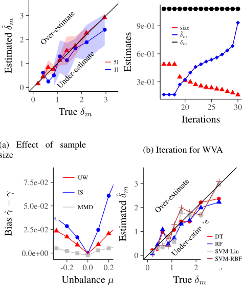
Results. First, we test whether Algorithm 1 identifies correctly the worst-case violation that occurs in the sub-space {(x1, x2)|x21 + x22 ≤ 1 and y = -1}. mdfa is trained using a support vector machine (RBF kernel) on a unbalanced data (µ = 0.2) with value of δm varying from 0 to 3.0. Figure 1a plots the estimated ˆ δm against the true one δm and shows that mdfa's estimate ˆ δm is unbiased. Figure 1b shows that at each iteration of the Algorithm 1, the estimated worstcase violation ˆ δm progresses toward the true value δm. Secondly, we compare our balancing approach MMD to alter-
(c) Effect of imbalance
(d) Choice of auditor class C
Figure 1: Performance of mdfa on synthetic data. If not precised otherwise, mdfa is trained with a support vector machine with 5K samples and imbalance factor µ = 0.2
native re-balancing approaches: (i) uniform weights (UW) with u(x) = 1/m for all x and (ii) importance sampling (IS) with exact weights w(x). UW applies mdfa without rebalancing. IS uses oracle access to the importance sampling weights w, since they are known in this synthetic experiment. Figure 1c plots the bias ˆ γ - γ for each unfairness certificate obtained by mdfa with varying values of the imbalance factor µ. It shows that minimizing the maximum-mean discrepancy function is the only method that generates unbiased certificates regardless of data imbalance. Bias in estimates obtained with UW confirms that absent of a re-weighting scheme, mdfa cannot disentangle the information related to S leaked by the features x from the one leaked by the classifier's outcomes y. Using importance sampling weights (IS) directly does not perform well: this confirms previous observations in the literature that in finite sample, the variance of the importance sample weights can be detrimental to a re-balancing approach. Lastly, Figure 1d shows that mdfa's estimates of δm are robust to diverse classes of classifiers, including support vector machines with non-linear SV M -RBF or linear SV M - Lin kernels and random forest RF .
4.2 Case Study: COMPAS
We apply our method to the COMPAS algorithm, widely used to assess the likelihood of a defendant to become a recidivist Proceedings of the Twenty-Eighth International Joint Conference on Artificial Intelligence (IJCAI-19)
| Variable | Population | Violation | ||
|---|---|---|---|---|
| AA | Other | AA | Other | |
| Prior Felonies | 4.44 (5.58) | 2.46 (3.76) | 0.79 (0.24) | 0.67 (0.17) |
| Charge Degree | 0.31 (0.46) | 0.4 (0.49) | 0.74 (0.23) | 0.74 (0.2) |
| Juvenile Felonies | 0.1 (0.49) | 0.03 (0.32) | 0.01 (0.02) | 0.0 (0.02) |
| Juvenile Misdemeanor | 0.14 (0.61) | 0.04 (0.3) | 0.01 (0.02) | 0.01 (0.01) |
| High Risk | 0.14 (0.35) | 0.05 (0.22) | 0.06 (0.04) | 0.02 (0.01) |
([ProPublica, 2016]). The research question is whether without knowledge of the design of COMPAS, mdfa can identify group of individuals that could argue for a disparate treatment. The data collected by ProPublica in Broward County from 2013 to 2015 contains 7K individuals along with a risk score and a risk category assigned by COMPAS. We transform the risk category into a binary variable equal to 1 for individuals assigned in the high risk category (risk score between 8 and 10). The data provides us with information related to the historical criminal history, misdemeanors, gender, age and race of each individual.
Worst Violations. We run mdfa on 100 different 70/30% train/test splits and report average value of auditing features and recidivism risk for the whole population and the worstcase subpopulation in Table 1. The first two columns show that the distribution of features in the whole population is disperse and differs between African American (AA) and Other. This is due to the data imbalance issue (c.f. Section 3). The probability of being classified as high risk is 0.14 for AfricanAmerican, thereby 2.7 times higher than for non-African American. However, it is unclear whether that difference could be explained either by the distribution imbalance or by the classifier's disparate treatment. The two last columns in Table 1 show that in the sub-population "violation" extracted by mdfa, the distribution of features is narrower and similar for African-American and non-African American: the subpopulation is made of individuals with little criminal and misdemeanor history. However, African American are still three times more likely to be classified as high risk. A policy implication of mdfa findings is that a judge using COMPAS may discount its assessment for African-American with little criminal history.
4.3 Group Fairness vs. Multi-Differential Fairness
We evaluate whether previous fairness correcting approaches protect small group of individuals against violation of differential fairness. We consider two techniques: (i) [Feldman et al., 2015]'s disparate impact with a logistic classification (DI - LC) and (ii) [Agarwal et al., 2018]'s reduction with a logistic classification (Red - LC). We use mdfa to identify sub-population G with worst-case violations and measure disparate treatment as DTG = Pr[Y = 1|S = 1,G]/Pr[Y = 1|S = -1,G]. We compare DTG to its aggregate counterpart computed on the whole population DI = Pr[Y = 1|S = 1]/Pr[Y = 1|S = -1].
| Repair | Adult | German | Crimes | |||
|---|---|---|---|---|---|---|
| Technique | DTG | DI | DTG | DT | DTG | DI |
| LC | 1.88 (0.4) | 1.08 | 1.26 (0.14) | 1.07 | 5.76 (3.16) | 1.0 |
| DI-LC | 1.44 (0.32) | 0.99 | 1.1 (0.08) | 1.04 | 5.74 (2.19) | 1.0 |
| Red-LC | 1.6 (0.25) | 1.03 | 1.04 (0.21) | 1.01 | 5.24 (0.89) | 1.0 |
Data. The experiment is carried on three datasets from [Friedler et al., 2018; Kearns et al., 2018]): Adult with 48840 individuals; German with 1000 individuals; and, Crimes with 1994 communities. In Adult the prediction task is whether an individual's income is less than 50K and the sensitive attribute is gender; in German, the prediction task is whether an individual has bad credit and the sensitive attribute is gender; in Crimes, the task is to predict whether a community is in the 70th percentile for violent crime rates and the sensitive attribute is whether the percentage of African American is at least 20%. For each data, each repair technique produces a prediction; then, mdfa is trained on 70% of the data and computes estimates for disparate treatment DTG on the remaining 30% of the data. The experiment is repeated with 100 train/test splits.
Results. In Table 2, even despite the fairness correction applied by DI - LC and Red - LC, mdfa still finds subpopulations G for which DTG is significantly larger than one. It indicates the existence of group of individuals who are similar but for their sensitive attributes and who are treated differently by the classifier trained by either DI-LC or Red-LC. The repair techniques reduce the aggregate disparate impact compared to the baseline (LC), since DI is closer to one for DI - LC and Red - LC across all datasets. However, in the Adult dataset, DTG remains between 1.44 and 1.6 after repair: mdfa identifies a group G of Females that are 44%-60% more likely to be of low-income than Males with similar characteristics. In Crimes dataset, disparate treatment DTG is around 5.7 for both DI -LC, R-LC: this means that there exist communities with dense African-American populations that are six times more likely to be classified at high risk than similar communities with lower percentages of African Americans.
5 Conclusion
In this paper, we present mdfa, a tool that measures whether a classifier treats differently individuals with similar auditing features but different sensitive attributes. We hope that mdfa's ability to identify sub-populations with severe violations of differential fairness could inform decision-makers when to discount the classifier's outcomes. It also provides the victims with a framework to contest a classifier's outcomes.
Avenues for future research are to investigate (i) the properties of a classifier trained under a multi-differential fairness constraint; and, (ii) the possibility to extend our approach to re-balance distributions in order to make counterfactual inference [Johansson et al., 2016] in the context of algorithmic fairness.
Acknowledgements
This work is partially supported by the National Science Foundation grant #1447489.
A Appendix: Proofs
Lemma 3.1.
Proof. Denote 〈x, x′ 〉 the inner product between x and x′ . Observe that for r = ± the left-hand side in Eq. (4) can be written 1 2 〈 c+1 2 , S 1+rY 2 〉 since 〈x, x′ 〉 = Prw[x = x′ ] - 1 for any x, x′ ∈ {-1, 1}. The result from lemma 3.1 follows by remarking that 〈S, 1〉 = 〈S, c〉 = 2Prw[S = c] - 1 = 0, since Prw[S = s|x] = Prw[S ̸= s|x].
Theorem 3.2.
Proof. (i) ⇒ (ii). Denote (xi, si, oi) a sample from a balanced distribution D over X × S × {-1, 1}. Denote c∗ ∈ C such that Pr[c∗ (xi) = oi] = maxc∈CPr[c(xi) = oi] = opt. Construct a function f such that for (xi, si, oi), f(xi, si) = sioi. Therefore, f(xi)si = oi and Pr[c∗ = sif(xi)] = Pr[c∗ = oi] = opt: by lemma 3.1, c∗ is a γ-unfairness certificate, with γ = opt+ρ-1 4 and ρ = Pr[oi = 1]. By (i), the certifying algorithm outputs a (γ - ϵ/4)- unfairness certificate c ∈ C with probability 1 - η and O(log(|C, log( 1 η ), 1 ϵ2 ) sample draws. Hence, by lemma 3.1, Pr[c(xi) = oi] = Pr[c(xi) = f(xi)oi] = 4(γ - ϵ/4) + 1 - ρ = opt - ϵ, which concludes (i) ⇒ (ii)
(ii) ⇒ (i). Suppose that f is a γ-unfair. Denote yi = f(xi, si). Samples {(xi, si), yi} are drawn from a balanced distribution over X × S × {-1, 1}. By lemma 3.1, there exists c ∈ C such that Pr[c(xi) = siyi] = 4γ + 1 - ρr, with r = ±. Assume, without loss of generality r = +. Then, since maxc′ Pr[c(xi) = siyi] ≥ 4γ + 1 - ρ+. By (ii), there exists an algorithm that outputs with probability 1-η and O(log(|C, log( 1 η ), 1 ϵ2 ) sample draws c ∈ C such that Pr[c(xi) = siyi] ≥ maxc′ Pr[c(xi) = siyi] - ϵ/4. Therefore Pr[c(xi) = siyi] ≥ 4(γ - ϵ) + 1 - ρ+. By lemma 3.1, c is a (γ - ϵ)- unfairness certificate for f, which concludes (ii) ⇒ (i).
Theorem 3.4. We first show the following lemma
Lemma A.1. With the same assumption as in lemma 3.3, for any weights u, w, ||u - w|| ≤ Gk(u, w)/√λmin(k), where λmin(k) is the smallest eigenvalue of the Gram matrix associated with k
Proof. First, note that Gk(u,w) = √(u-w)T k(u-w) and by a standard bound on Rayleigh quotient, ||u - w|| ≤ Gk(u, w)/√λmin(k).
Now we prove lemma 3.3:
Proof. The proof relies on the fact that the solution of Eq. (5) is distributionally stable as in [Cortes et al., 2008]:
where λmax(k) is the largest eigenvalue of the Gram matrix associated to k (see [Cortes et al., 2008], proof of theorem 1). Moreover, |hu(x) - hw(x)| ≤ ||hu - hw||k. The result in lemma 3.3 follows from lemma A.1 and cond(k) = λmax(k)/λmin(k).
The next result follows from [Gretton et al., 2009] and bounds above ˆGk(u,ws), the emprical counterpart of Gk(u, ws), where ws(x) = P r[S ̸= s|x]/(1 - P r[S = s|x]) are the importance sampling weights for S = s.
Lemma A.2. Let η > 0. Denote ns = |{i = 1, ...,m|si = s}| and ns = |{i = 1, ...,m|si ̸= s}|. Suppose that ||u||∞ < B/ns and that E[u] < ∞. There exists a constant κ1 > 0 such that with probability 1 - η,
.
For τ > 0, we construct c ∈ C from the real-valued function h as
Lemma A.3. Let τ, η > 0, ϵ > 0. Let ˆ cu, ˆ cw denote the certificates constructed from the solution of the empirical risk minimization ˆhu (with weights u) and ˆhw (with weights ws). There exists κ2 > 0 such that with probability 1 - η,
.
κ2 = κ1κσ2 2λc . By lemma 3.3 and lemma A.2, ||ˆhu - ˆhw||2 ≤ ϵm with probability 1 - η. Consider first the case ˆhw < -τ . Then, with probability 1 - η, {xi|ˆ cu(xi) ̸= ˆ cw(xi) ∧ ˆhw(xi) < -τ} = {xi|(-τ + ϵm > ˆhu(xi) > -τ ) ∧ (ˆ cu(xi = 1) ∧ ˆhw(xi) < -τ] by lemma 3.3. Therefore, by construction of ˆ cu, |{xi|ˆ cu(xi) ̸= ˆ cw(xi)∧ˆhw(xi) < -τ}| = m τ+hu 2τ ≤ m ϵm 5τ . A similar result is obtained for ˆhw > τ. .
Lastly, with probability 1 - η, |{xi|ˆ cu(xi) ̸= ˆ cw(xi) ∧ ˆhw(xi) ∈ (-τ, τ )}| ≤ 2m ϵm 5τ +m |hu-hw| τ ≤ 3 ϵm 5τ . The first part of the inequality uses the results obtained in the previous paragraph for |ˆhu| > τ; the second part uses the construction of ˆ cu and ˆ cw. Therefore, with probability 1 - η, |i=1,...,m|ˆ cu(xi)̸=ˆ cw(xi)| m ≤ 5ϵ(m)/τ.
Lemma A.4. Consider a random variable Z and ˆ cu, ˆ cw as in lemma A.3. Then |Pr[Z = 1 ∧ ˆ cu = 1] - P r[Z = 1 ∧ ˆ cw = 1]| ≤ Pr[ˆ cu ̸= ˆ cw]
The last result we need to prove theorem 3.4 is to link ns and n¬s to sample size m
Proof. This is an application of a Hoeffding's inequality for Bernouilly random variable.
The proof of theorem 3.4 then follows from the fact that for a sample balanced with weights u, ˆ γu = Pr[ˆ cu = 1] ( eδu eδu+1 - 12 ) with eδu = Pr[Y = 1|S = 1, ˆ cu = 1]/Pr[Y = 1|S = -1, ˆ cu = 1]. By lemmas A.4 and A.5, for any ϵ′ > 0 with Ω ( 1 (ϵ′ )2α2s log 2 η ) samples, with probability 1-η, |eδu -eδw | < ϵ′ and |Pr[ˆ cw = 1∧Y = 1]-Pr[ˆ cu = 1 ∧ Y = 1]| ≤ ϵ′ . There exists κ3 such that for ϵ > 0, with probability 1 - η, |ˆ γu - ˆ γw| ≤ κ3ϵ. Moreover, by theorem 3.2, if C has finite VC dimension, with probability 1 - η and Ω (log(|C|), 1 ϵ2 , log 2 η ) samples, |ˆ γw - γw| ≤ ϵ. It follows that with probability 1-η andΩ (log(|C|), 1 ϵ2α2s , log 2 η ) samples, |ˆ γu - γw| ≤ (1 + κ3)ϵ. That concludes the proof since by lemma 3.1, if f is γ-unfair, then γ = γw.
Theorem 3.5. Assume that the classifier f is γ-unfair for Y = y ∈ {-1, 1}. Let δm denote the worst-case violation. Note that by definition of γ and δm: γ = α ( eδm eδm+1 - 1 2 ). At each iteration t, denote ct the solution of the following optimization problem
where uit are the weights at iteration t and the expectation is taken over all the samples of size m drawn from Df .
Lemma A.6. Let s ∈ S. Assume that the classifier f is γunfair. At iteration t, denote δt = ln(Pr[Y = 1|ct(x) = 1, S = s]/Pr[Y = 1|ct(x) = 1, S = s]). Then, eδt 1+eδt ≥ 1 - h(ξt), where h(ξt) = 4γ+1-2ρ+ ξt .
Proof. Without loss of generality, we assumey = 1. Denote c-1 such that c-1(x) = -1 for all x. By comparing the value of the empirical risks for ct and c-1, if ct ̸= c-1, then we can show that
Moreover,
It follows that if ct ̸= c-1, since Pru[ct = 1, Y = y] ≥ α Pru[SY = ct|ct = 1, Y = y] ≥ 1 - 1 αξt (Pru[ct = SY )] - ρ+). Since the classifier f is γ-unfair for y = 1, we know that maxc∈C Pru[SY = c] = 4γ + 1 - ρ+. Therefore, at iteration t, either ct = c-1 or
Since y = 1, Pru[Y = 1|ct = 1, S = 1] ≥ 1 - h(ξt). Without loss of generality, we can assume Pr[Y = 1|ct = 1, S = 1] ≥ 1 - h(ξt). It follows that eδt ≥ 1-h(ξt) h(ξt) .
Lemma A.7. Denote T = 4γ+1-2ρ(y) ξα (eδm + 1). The algorithm stops for t ≥ T with Pr[Y = y,Ct = 1] = α and δt = δm.
Proof. First, note that h(ξT) = 1 eδm+1 and thus that δT ≥ δm. Moreover, at iteration t, ct is chosen over cm where cm is the sub-population that corresponds to the worst-case violation δm. Comparing the expected risk for cm and ct at iteration t leads to
By definition of the worst-case violation for y = 1, Pru[SY ̸= ct|ct = 1, Y = 1] ≥ Pru[SY ̸= cm|cm = 1, Y = 1]. Moreover, when the algorithm stops, Pru[ct = 1, Y = 1] = α = Pru[cm = 1, Y = 1]. Therefore, the right-hand side of (11) is non-negative. It results that Pru[SY = ct] ≥ Pru[SY = cm]. On the other hand, since f is γ- unfair, Pru[SY = ct] cannot be more than 4γ - ρ+ + 1. Therefore, P ru[SY = ct] = 4γ - ρ+ + 1.
It follows that at iteration t, when the algorithm stops
The algorithm stops when Pr[Y = 1, ct = 1] = α, which implies δt = δm. Therefore, t ≤ T .
@inproceedings{ijcai2019p814,
  title     = {mdfa: Multi-Differential Fairness Auditor for Black Box Classifiers},
  author    = {Gitiaux, Xavier and Rangwala, Huzefa},
  booktitle = {Proceedings of the Twenty-Eighth International Joint Conference on
               Artificial Intelligence, {IJCAI-19}},
  publisher = {International Joint Conferences on Artificial Intelligence Organization},
  editor    = {Sarit Kraus},
  pages     = {5871--5879},
  year      = {2019},
  month     = {8},
  note      = {AI for Improving Human Well-being},
  doi       = {10.24963/ijcai.2019/814},
  url       = {https://doi.org/10.24963/ijcai.2019/814},
}
TY - CPAPER TI - mdfa: Multi-Differential Fairness Auditor for Black Box Classifiers AU - Gitiaux, Xavier AU - Rangwala, Huzefa T2 - Proceedings of the Twenty-Eighth International Joint Conference on Artificial Intelligence, IJCAI-19 PB - International Joint Conferences on Artificial Intelligence Organization PY - 2019 SP - 5871 EP - 5879 DO - 10.24963/ijcai.2019/814 UR - https://doi.org/10.24963/ijcai.2019/814 ER -Copied
Machine-readable versions of this paper, for tools and AI agents:





