
Bayesian Parameter Estimation for Nonlinear Dynamics Using Sensitivity Analysis
Proceedings of the Twenty-Eighth International Joint Conference on Artificial Intelligence. Main track. Pages 5708-5714.
https://doi.org/10.24963/ijcai.2019/791
Keywords
- Machine Learning: Learning Generative Models
- Uncertainty in AI: Approximate Probabilistic Inference
Abstract
We investigate approximate Bayesian inference techniques for nonlinear systems described by ordinary differential equation (ODE) models. In particular, the approximations will be based on set-valued reachability analysis approaches, yielding approximate models for the posterior distribution. Nonlinear ODEs are widely used to mathematically describe physical and biological models. However, these models are often described by parameters that are not directly measurable and have an impact on the system behaviors. Often, noisy measurement data combined with physical/biological intuition serve as the means for finding appropriate values of these parameters.
Our approach operates under a Bayesian framework, given prior distribution over the parameter space and noisy observations under a known sampling distribution. We explore subsets of the space of model parameters, computing bounds on the likelihood for each subset. This is performed using nonlinear set-valued reachability analysis that is made faster by means of linearization around a reference trajectory. The tiling of the parameter space can be adaptively refined to make bounds on the likelihood tighter. We evaluate our approach on a variety of nonlinear benchmarks and compare our results with Markov Chain Monte Carlo and Sequential Monte Carlo approaches.
- [Bak and Duggirala, 2017] Stanley Bak and Parasara Sridhar Duggirala. Hylaa: A tool for computing simulation-equivalent reachability for linear systems. In HSCC, pages 173-178. ACM, 2017.
- [Benavoli and Piga, 2016] Alessio Benavoli and Dario Piga. A probabilistic interpretation of set-membership filtering: Application to polynomial systems through polytopic bounding. Automatica, 70:158-172, 2016.
- [Berz and Makino, 1998] M. Berz and K. Makino. Verified integration of ODEs and flows using differential algebraic methods on high-order Taylor models. Reliable Computing, 4:361-369, 1998.
- [Berz, 1999] Martin Berz. Modern Map Methods in Particle Beam Physics, volume 108 of Advances in Imaging and Electron Physics. Academic Press, 1999.
- [Chen et al., 2012] Xin Chen, Erika Ábrahám, and Sriram Sankaranarayanan. Taylor model flowpipe construction for non-linear hybrid systems. In Proc. RTSS'12, pages 183-192. IEEE, 2012.
- [Chen et al., 2013] Xin Chen, Erika Ábrahám, and Sriram Sankaranarayanan. Flow*: An analyzer for non-linear hybrid systems. In Proc. of CAV'13, volume 8044 of LNCS, pages 258-263. Springer, 2013.
- [Coelho et al., 2011] Flávio Coelho, Cláudia Codeco, and M. Gabriela M. Gomes. A bayesian framework for parameter estimation in dynamical models. PLoS ONE, 6, 2011.
- [Dempster, 1967] A.P. Dempster. Upper and lower probabil- ities induced by a multivalued mapping. The Annals of Mathematical Statistics, 38(2):325-339, 1967.
- [Doucet et al., 2001] Arnaud Doucet, Nando De Freitas, and Neil Gordon. Sequential Monte Carlo Methods in Practice. Springer, 2001.
- [Enszer et al., 2011] J.A. Enszer, Y. Lin, S. Ferson, G.F. Corliss, and M.A. Stadtherr. Probability bounds analysis for nonlinear dynamic process models. AIChE Journal, 57:404-422, 2011.
- [Ferson et al., 2003] Scott Ferson, Vladik Kreinovich, Lev Ginzburg, David S. Myers, and Kari Sentz. Constructing probability boxes and dempster-shafer structures. Technical Report SAND2002-4015, Sandia Laboratories, January 2003.
- [Ferson, 1996] Scott Ferson. What Monte-Carlo methods cannot do. Human and Ecological Risk Assessment, 2:990-1007, 1996.
- [Fox, 2009] Emily B. Fox. Bayesian Nonparametric Learning of Complex Dynamical Phenomena. PhD thesis, MIT, 2009.
- [Girolami, 2008] Mark Girolami. Bayesian inference for differ- ential equations. Theoretical Computer Science, 408(1):4 - 16, 2008. Computational Methods in Systems Biology.
- [Goodman and Stuhlmüller, 2014] Noah D Goodman and Andreas Stuhlmüller. The Design and Implementation of Probabilistic Programming Languages. http://dippl.org, 2014. Link
- [Goodman et al., 2008] Noah D. Goodman, Vikash K. Mans- inghka, Daniel M. Roy, Keith Bonawitz, and Joshua B. Tenenbaum. Church: a language for generative models. In Uncertainty in Artificial Intelligence, pages 220-229, 2008.
- [Halpern, 2005] Joseph Y. Halpern. Reasoning about Uncer- tainty. MIT Press, 2005.
- [Kapela et al., 2010] T. Kapela, M. Mrozek, P. Pilarczyk, D. Wilczak, and P. Zgliczynski. CAPD -a rigorous toolbox for computer assisted proofs in dynamics. Technical report, Jagiellonian University, 2010.
- [Makino and Berz, 2003] Kyoko Makino and Martin Berz. Tay- lor models and other validated functional inclusion methods. J. Pure and Applied Mathematics, 4(4):379-456, 2003.
- [McElreath, 2015] Richard McElreath. Statistical Rethinking: A Bayesian Course with Examples in R and Stan. CRC Press, 2015.
- [Milanese and Novara, 2009] Mario Milanese and Carlo Novara. Set membership methods in identification, prediction and filtering of nonlinear systems. IFAC Proceedings Volumes, 42(10):263-272, 2009.
- [Mooij and Kappen, 2009] Joris M Mooij and Hilbert J Kappen. Bounds on marginal probability distributions. In NeurIPS, pages 1105-1112, 2009.
- [Nedialkov, 2006] Ned S. Nedialkov. Interval tools for ODEs and DAEs. 2006.
- [Nelles, 2001] Oliver Nelles. Nonlinear System Identification. Springer, 2001.
- [Radul, 2007] Alexey Radul. Report on the probabilistic language scheme. In DLS, pages 2-10. ACM, 2007.
- [Robert and Casella, 1999] Christian P. Robert and George Casella. Monte Carlo Statistical Methods. Springer, 1999.
- [Robert, 2016] Christian P. Robert. Monte Carlo Methods. John Wiley & Sons, 2016.
- [Roux et al., 2016] Pierre Roux, Yuen-Lam Voronin, and Sriram Sankaranarayanan. Validating numerical semidefinite programming solvers for polynomial invariants. In Static Analysis Symposium, volume 9837 of LNCS, pages 424-446. Springer, 2016.
- [Shafer, 1976] Glenn Shafer. A Mathematical Theory of Evidence. Princeton University Press, 1976.
- [Shmarov and Zuliani, 2015] Fedor Shmarov and Paolo Zuliani. Probreach: verified probabilistic delta-reachability for stochastic hybrid systems. In HSCC'15, pages 134-139, 2015.
- [Söderström and Stoica, 1989] T. Söderström and P. Stoica. System Identification. Prentice Hall, Upper Saddle River, N.J., 1989.
- [Vanlier et al., 2013] J. Vanlier, C.A. Tiemann, P.A.J. Hilbers, and N.A.W. van Riel. Parameter uncertainty in biochem- ical models described by ordinary differential equations. Mathematical Biosciences, 246(2):305 -314, 2013.
- [Wang and Elhag, 2006] Ying-Ming Wang and Taha MS Elhag. On the normalization of interval and fuzzy weights. Fuzzy sets and systems, 157(18):2456-2471, 2006.
- [Wood et al., 2014] Frank Wood, Jan Willem van de Meent, and Vikash Mansinghka. A new approach to probabilistic program- ming inference. In Proc. AISTATS'14, pages 1024-1032, 2014.
References were extracted automatically from the PDF and may contain errors.
Full text extracted automatically from the PDF; figures, tables and equations may differ. The PDF is the version of record.
1 Introduction
In this paper, we study the problem of inferring posterior probabilities of parameters of ODE models. ODE models are common in numerous scientific applications and often, they involve parameters whose values are to be estimated from given observation data. Our approach considers ODEs with unknown parameters over which a prior distribution is defined. We then condition this model on noisy observations over time, to compute a posterior distribution using the Bayes rule. Such estimation has been studied across numerous scientific and engineering disciplines. Common approaches include the use of Monte-Carlo methods [Robert and Casella, 1999; Doucet et al., 2001; Robert, 2016] such as Markov Chain Monte Carlo (MCMC) and Sequential Monte Carlo (SMC). MCMC approaches perform a random walk over the space of parameters using a carefully designed transition kernel whose invariant distribution matches the desired posterior that we wish to sample from [Robert and Casella, 1999]. On the other hand, particle filters (a prototypical SMC approach) uses numerous particles which are periodically resampled in proportion to their likelihoods [Doucet et al., 2001]. These approaches produce samples that converge in distribution to the actual posterior in the limit, provided they are run long enough (for MCMC approaches) or sufficiently many particles are chosen (for particle filters). In this paper, we examine an approach that uses imprecise probability models for the posterior distributions in the form of probability intervals defined over a decomposition of the parameter space. Such models can be complementary to sampling-based approaches described previously [Ferson, 1996].
The key idea is to iteratively partition the space of parameters into finitely many cells, and find interval bounds on the posterior likelihood for each cell. The likelihood bounds can be normalized and as a result, we produce bounds on the posterior probability of each cell. The result of our approach is an imprecise probability distribution that takes on the same form as Dempster-Shafer structures or p-boxes [Halpern, 2005; Ferson et al., 2003; Dempster, 1967; Shafer, 1976]. Once the likelihood bounds are produced for a coarse partition of the parameter space, we can further refine cells whose upper and lower bounds are far apart to improve the approximation of the posterior.
We evaluate our approach on a series of benchmarks ranging from 2-6 parameters, comparing the results from our approach with those obtained from a sufficient number of MCMC and SMC simulations for each benchmark. The results show that our approach yields an accurate description of the posterior distribution but at the same time suffers from the curse of dimensionality beyond 6 parameters.
1.1 RelatedWork
The problem of finding parameters of a dynamical system that fit given data has been the subject of much work in the fields of system identification [Nelles, 2001; S¨oderstr¨om and Stoica, 1989]. Broadly, the approaches fall into two categories: (a) approaches that attempt to find parameters that minimize a loss function such as least squares that measures the disagreement between the model predictions and the actual data; and (b) approaches that use a prior distribution over the parameters and use Bayes rule to compute a posterior given the data [McElreath, 2015]. Beyond applications to control, the Bayesian approach has been applied to perform parameter inference for biological models [Girolami, 2008;
Coelho et al., 2011; Vanlier et al., 2013]. Recently, the convergence of programming languages and Bayesian inference methods has led to the area of probabilistic programming, wherein executable programs are used as models conditioned on observation data [Goodman et al., 2008; Goodman and Stuhlm¨uller, 2014; Radul, 2007; Wood et al., 2014]. Our future work will explore extensions of these languages by adding support for continuoustime dynamics to tackle applications hybrid cyber-physical systems. In this context, Bayesian inference approaches for linear hybrid models have been well-studied (Cf. [Fox, 2009]).
Our approach uses ideas from reachability analysis of nonlinear ODEs. Given a set of initial states and parameters, reachability analysis computes a guaranteed over-approximation of the reachable set of states at time t. Numerous approaches exist to compute reachable set approximations efficiently for large linear systems with tens of thousands of state variables [Bak and Duggirala, 2017]. For nonlinear systems, however, the problem is much harder. However, recent advances using higher order interval analysis approaches have shown much promise, leading to tools such as VNODE-LP [Nedialkov, 2006], COSY-INFINITY [Berz, 1999; Makino and Berz, 2003], CAPD [Kapela et al., 2010], and Flow* [Chen et al., 2013]. Interestingly, our experience in this paper shows that such rigorous approaches are often prohibitively expensive for Bayesian inference since they need to be run repeatedly over many different subsets of parameters. In this paper, we use a sensitivity analysis approach based on numerical simulations to perform an approximate but inexpensive reachability analysis.
In our paper, we employ an imprecise probability model similar to Dempster-Shafer structures that provide upper and lower bounds on the likelihoods to cells in the parameter space [Dempster, 1967; Shafer, 1976; Ferson et al., 2003]. We normalize these likelihood bounds to obtain bounds on probabilities. The idea of using imprecise probabilities to explore uncertainty is not new. Mooij et al represent the marginal probability for each variable using a box over the set of measures for graphical models with discrete random variables [Mooij and Kappen, 2009]. Our approach focuses solely on ODE models rather than graphical models with only discrete variables. Secondly, we focus on representing the joint posterior as a set of measures rather than just the marginals over each individual random variable, and finally we provide a hierarchical box partitioning scheme to avoid the problem of the uniformly sized grids, and thus enhance scalability.
Enszer et al used a combination of reachability analysis and the decomposition of the parameter space into cells to propagate a given distribution over initial states and parameters forward in time, thus obtaining an imprecise probability distribution at a future time point [Enszer et al., 2011]. The key difference is that our approach conditions the result of the reachability analysis on observation data, whereas Enszer et al focus on uncertainty propagation. Likewise Shmarov et al use reachability as part of the tool ProbReach [Shmarov and Zuliani, 2015] but treat the "forward model" without conditioning on data. Milanese et al present set-valued approaches for system identification - the problem of deriving a functional form of a dynamical system from observations [Milanese and Novara, 2009]. However, their approach avoids the use of regression or parameterization of the dynamics, focusing instead on interval bounds over the unknown function. Benavoli et al also define the set of possible posteriors using a semi-infinite LP, that uses the classic Lassere's moment problem to reduce to a Sum-of-square (SOS) polynomial optimization [Benavoli and Piga, 2016]. It can be used to infer unknowns such as bounds on the posterior moments and posterior probabilities in certain regions. However, their approach is limited when addressing the nonpolynomial systems. Our approach is found capable of dealing with nonpolynomial systems by performing sensitivity analysis. Although SOS programs are solved by reduction to convex semidefinite optimization problems (SDP), the relaxation can involve high degree polynomials that in turn lead to large SDPs. Numerical issues have been commonly observed [Roux et al., 2016].
2 Preliminaries
We consider dynamical systems S defined by a system of ODEs dx dt =f(x,p) over state space x∈Rn, and a parameter space p∈ P. Let the number of parameters be given by np≥1. Fixing the parameters p∈P, a trajectory of the system starting from initial state x(0) at time t=0, is defined as a function x : [0,T] ↦→Rn such that dx dt |(t=s) =f(x(s),p). Assuming that f is Lipschitz continuous in x and continuous in p, we obtain that the time trajectory x(t) is unique for fixed x(0) and p. Let us denote x(t) : SIM(x(0),p,t) as the state reached at time t≥0. Let us consider two illustrative examples, starting with a simple ball example.
Example 2.1. (Simple Ball Example) Consider a ball thrown into the air starting at initial position (0,0) and initial velocity (vx(0)=5,vy(0)=-4). Its motion is described by the equations
The state space is given by (x,y,vx,vy) and the single parameter is g.
Example 2.2. (Fitzhugh-NagumoModel) Consider the nonlinear Fitzhugh-Nagumo model for a neuron over states (x1,x2) with initial state (-1,1) and γ=0.5, involving parameters (θ1,θ2):
2.1 Observations, Priors and Bayesian Inference
Let S be a dynamical system over state space x and parameters p ∈ P defined by a vector field f(x,p). We define a prior distribution π over the parameter space P. For convenience, let π(p) denote the density function of the prior distribution over p∈P. We also assume that π is supported over P. Next, let g :Rn ↦→Rm be an output map from states x to output y : g(x). We assume that the outputs can be measured with an error e that is distributed as a zero mean normal random variable with variance σ2: e∼N(0,σ2Im×m). Let the samples be observed at some pre-specified times 0 < t1 < t2 ··· < tk, with k > 0 observations. The overall model is specified as follows:
Let Y : (y(t1),...,y(tk)) represent the observations. The goal is to compute posterior distributions over the parameters that factor in the observations and the prior. Recall that the posterior is defined as:
The left hand side is the posterior probability of p whereas the right hand side involves P(Y |p) which is the probability of observations Y for a specific value of parameter p, the prior distribution at p given by π(p). The denominator P(Y ) is a normalizing constant ∫P P(Y |p) π(p)dp. This is often called the evidence and equals the probability that the observations Y are obtained under the prior. Note that the posterior is well-defined only if P(Y )̸=0. We will assume this is the case throughout this paper. However, P(Y ) is difficult to compute, in general. As a result, we often consider the unnormalized likelihood function, the numerator of Eq. (1).
The goal of Bayesian inference is to obtain the posterior distribution P(p|Y ). The posterior distribution can be used to solve many problems:
- Sampling Problem: Obtain samples from the posterior distribution.
- PosteriorMean/Moments: Compute mean/moments from the posterior.
- Maximum A posteriori (MAP) Estimate: Obtain the parameter p that has maximum probability (density) under the posterior distribution.
- Property Checking: Estimate the probability that the system behaviors satisfy a property of interest, assuming parameters are sampled from the posterior.
Example 2.3. Going back to Example 2.1., let us add observations of the y-position to the model at times y1 =-9 at t1 =1 and y2=-31 at t2=2 seconds respectively. We assume that the sampling distribution is a Gaussian with zero mean and σ = 1. We seek to compute the posterior distribution of the parameter g, given these observations. The prior distribution for g is taken to be uniform over the interval g∈[7,12]. The reader will notice that no value of g explains the data perfectly. However, since we assume measurement errors, no value of g over the range can be ruled out as having zero The posterior likelihood of g can now be calculated using the formula
C is a normalizing constant obtained by calculating the integral: ∫ 12 7 exp(-2.125g2 +48.5g)dg.
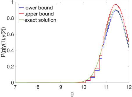
The reader may recognize the posterior distribution of g as a truncated Gaussian with a peak at g=11.41. Figure 1 shows the posterior distribution.
2.2 Monte Carlo SamplingMethods
Monte Carlo approaches seek to derive samples from the posterior. These approaches produce sample values p1,p2,...,pN such that as N →∞, the distribution of these samples converges to the posterior P(p|Y ). There are numerous Monte Carlo approaches. However, they can be generally categorized into two major classes: (a) Markov-Chain Monte Carlo (MCMC) methods and (b) Sequential Monte Carlo (SMC) approaches. Naturally, many approaches can be seen as a mix of MCMC and SMC. Details of these approaches, including their relative advantages/drawbacks are discussed in detail elsewhere [Robert and Casella, 1999; Robert, 2016; Doucet et al., 2001]. MCMC and SMC approaches are widely applicable, needing just repeated simulations of the model. However, both MCMC and SMC approaches produce parameter samples such that the distributions they sample from converge in probability to the true posterior in the limit as the number of samples goes to infinity. In this paper, we consider using reachability analysis and interval analysis to derive an approximation of the actual posterior.
3 Overall Approach
In this section, we provide a high-level overview of our approach. Rather than compute samples from the posterior, our approach seeks to represent the posterior in an abstract manner by bounding the measure associated with subsets of the parameter space P. Such an abstract representation will represent a family of probability distributions. Building on the soundness of the reachability analysis, we can provide a guarantee that the true posterior P(p|Y ) belongs to the family of distributions. The overall approach consists of three steps:
- Partition the parameter space P into cells C1,...,CK
- For each cell Ci, compute likelihood bounds [li,ui] for the posterior probability P(p∈Cj|Y ).
- Refine the approximation by further partitioning a subset of cells.
3.1 Partitioning
We first partition the parameter space P into a set of cells C1,...,CK such that ⋃Cj =P and furthermore, Ci∩Cj =∅ for i̸=j. This condition can be relaxed to allow Ci∩Cj to be a set of measure zero. Such a tiling can be obtained by gridding the parameter space and using half-open boxes to ensure that there are no intersections between adjacent cells. Moving forward, we assume that the cells C1,...,CK are fixed.
3.2 Computing Likelihood Bounds For a Cell
There are two steps in computing likelihood bounds for a cell Cj. (a) First, we perform a reachability analysis to bound the output at time ti as a function of the parameter value p for all p∈Cj. (b) Next, we will express the integral P(p∈Cj|Y ) and provide interval bounds on it. For each p∈Cj, let x(ti;p) denote the state reached at time ti; and y(ti;p) be the output obtained as g(x(ti;p)). The first idea is to express y(ti;p) as a polynomial over p plus an interval Ij,i.
The polynomial qj,i and the error interval are derived using reachability analysis approaches using Taylor model arithmetic and implemented in tools such as Flow* and COSY-INFINITY [Chen et al., 2012; 2013; Berz, 1999; Berz and Makino, 1998]. The main guarantee of the approach is that
Next, we compare the output y(ti;p) with the actual data yi. Since the sampling distribution is a Gaussian, we can write the posterior probability as the integral:
Here C is the normalization constant for the Gaussian distribution 1 (√2πσ2)k . Substituting y(ti;p) : qj,i(p)+Ij,i yields an integral that calculates the expectation of a polynomial over p plus an error interval over a box. As such, these integrals are hard to compute precisely. Therefore, we will need to bound the value of the integral in an interval [l,u]. A simple strategy to bounding integrals is to bound the integrand.
Lemma 3.1. Let ∏ki=1 [Cexp( ‖y(ti;p)-yi‖2 2σ2 )] ∈ [m,M] for all p∈Cj. The value of the integral from Eq. 3 is bounded by [mπ(Cj),Mπ(Cj)] wherein π(Cj) is the prior probability of the cell Cj .
Combining these bounds provides a representation of the unnormalized posterior likelihood L(p) : P(Y |p)π(p) over the parameter space P that associates upper and lower bounds with each cell Cj ⊆P .
Example 3.1. We will illustrate this on the simple ball example (Ex. 2.3.) which seeks to infer a parameter g∈[7,12] under the uniform prior. We partition the parameter space into five cells
Let us consider the cell C1. We know that the value of y(t) is given as y(t)=y0+vy(0)t- 1 2 gt2. Thus, we have
As a result, we obtain
| C1 | C2 | C3 |
|---|---|---|
| [2.6E-20,4.4E-13] | [4.4E-13,1.1E-7] | [1E-7,3.5E-4] |
| C4 | C5 |
|---|---|
| [3.5E-4,0.018] | [0.017,0.024] |
3.3 Normalization
Next, we will consider the problem of constructing a normalized distribution from the unnormalized model. Thus far, we have computed bounds [lj, uj], corresponding to the cell Cj, for j=1,...,K. This provides an interval for the unnormalized likelihood for each cell. Let W be a normalization constant P(Y )= ∫P P(Y |p)π(p)dp. A distribution D over P is compatible with the bounds [lj,uj] for each cell Cj iff PD(Cj)∈ 1W ([lj,uj]). Let unknowns pj ∈[0,1] represent the unknown probability PD(Cj) under some compatible distribution D. We have the constraint
wherein ˆW is a place holder for 1W Thus, we can formulate a linear program to compute bounds on the upper and lower probabilities for each cell and the constant W.
The LP can be solved analytically to yield the bounds [Wang and Elhag, 2006]
Besides minimizing/maximizing the probability of a cell, we can use the model to estimate bounds on the expectation of function h(p) over the parameters.
Example 3.2. Returning to Ex. 3.1., we note can compute bounds on the probability of cell C5 as
wherein ϵ≤0.001. The bounds are p5∈[0.48,0.986]. The bounds for the C4 are p4 ∈[0.014,0.514]. Cell C3 bounds are in the range [8.2×10-3,2.4×10-6]. The remaining cells have probabilities less than or equal to 10-5. The bounds are illustrated in Figure 1.
Thus, as we see in the example, a uniform decomposition often yields many cells with negligibly small probabilities and relatively fewer cells that carry the bulk of the probability. Thus, we need a refinement process that adaptively creates smaller sub cells to refine the approximation of the posterior.
3.4 Refining the Decomposition
The key drawback of our approach thus far is the need to decompose the parameter space, which makes the computational cost prohibitively expensive as the number of parameters grows. One approach to alleviate this lies in adaptively decomposing the parameter space. The adaptive decomposition is useful in many cases wherein large portions of the parameter space have very low posterior probabilities since they exhibit severe mismatches with the observed data. In these situations, a coarse approximation of these low probability regions combined with a finer abstraction of the higher probability regions yields a faster approach. To enable this approach, we choose an initial partition width ∆0. After partitioning the parameter space, we compute likelihood bounds for each cell, as described thus far. Next, we select a subset of the cells according to a refinement criterion. For this paper, we propose a refinement strategy that refines a cell Cj based on whether its difference in the log upper-bound likelihood uj from the maximum log upper-bound likelihood umax within a range W, i.e. logumax-loguj ≤W. The threshold W is chosen by trial and error for each benchmark example. Additionally, for a cell to be refined relative difference d= (u-l) u of the likelihood interval [l,u] must be smaller than the threshold d. In our evaluation, the relative difference is chosen to be 0.1. Other refinement strategies could include selecting cells with maximum uncertainty width (uj -lj); or using samples from a numerical Monte-Carlo scheme to select cells according to the decreasing order of the number of samples drawn inside each cell. Once a cell is chosen, it is further decomposed into smaller sub-cells and the entire process is repeated.
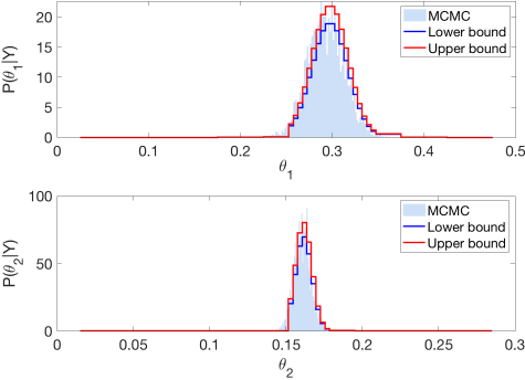
Example 3.3. (Fitzhugh-Nagumo Model Posterior) We will consider the Fitzhugh-Nagumo model from Ex. 2.2.. We fix the nominal parameters to θ1 = 0.3 and θ2 = 0.15 and create simulations. Now, we set the parameter space to be θ1 ∈ [0,0.5],θ2 ∈[0,0.3]. The posterior bounds are shown in Figure 2.
3.5 Rapid ExplorationUsing Sensitivity Analysis
Thus far, we have used ideas from reachability analysis to infer likelihood bounds on cells. However, in practice, running reachability analysis for each cell can be quite expensive, since these approaches attempt to maintain error intervals within specified ranges by taking even smaller steps over time or increasing the degree of the Taylor model. As a result, we find that existing solvers rapidly exhaust computational resources at the very first step which involves coarse refinement of P.
We can however achieve a speedup using sensitivity analysis to find a linear mapping between the parameter values and the outputs y(ti;p) for the current cell Cj. To achieve this, we proceed as follows:
- We compute a Jacobian matrix J(pj,ti) = ∂y(ti) ∂p |p=pj around a center point pj chosen in cell Cj. This allows us to approximate the effect of a perturbation pj+δ:
- We use Eq (5) rather than a sound Taylor model approximation as shown in Eq. (2) in order to obtain a rapid approximation of the likelihood bounds according to Eq (3).
The use of an unsound approximation is motivated by two important considerations: (a) For cells Cj that have a very low likelihood in the posterior, an approximation of the trajectory suffices to note that the bounds are quite coarse. (b) On the other hand, since we repeatedly refine the cells Cj that have larger likelihoods, although the bounds obtained are inaccurate for large cells due to the linearization error, the refinement to smaller cells makes the linearization quite precise and can bring the error to within acceptable limits. As a result, we use linear sensitivity analysis rather than sound reachability analysis to rapidly compute reachable state estimates for each cell Cj.
4 Experiments
We have implemented the ideas presented thus far in the C++ programming language using the ODEINT ODE solver. Our implementation uses the adaptive refinement strategy presented in Section 3. A detailed description of the benchmarks will be made available in the future as an extended technical report. Table 1 shows the benchmarks and the number of parameters considered for each benchmark as well as the number of state variables in the model. For each benchmark a "ground truth" parameter value, given in Table 1, was fixed to generate simulations from a fixed initial condition. One of the state variables is taken to be the output and thus the data is generated. The sampling distribution is taken to be a zero mean Gaussian distribution whose variance is adjusted based on the magnitude of the outputs.
Table 1 presents the computation time and the expectation E(p) of the parameters. The expectation of the posterior obtained from our approach is computed using the upper bounds of the probability of each cell and the center point pj of cell Cj as its nominal parameter value: ∑j P(p∈Cj |Y )uppj ∑j P(p∈Cj|Y )up . We compare this against the expectations obtained from the MCMC and SMC samples, noting that the computed values are nearly identical in all cases. This agreement serves to quantify the precision that can be derived from our approach.
| Benchmark | n,np | Time(s) of DSA | E(p)DSA | Time(s) of MCMC | NMCMC | E(p)MCMC | NSMC | E(p)SMC | Ground truth |
|---|---|---|---|---|---|---|---|---|---|
| FITZHUGH-NAGUMO | |||||||||
| model-1 model-2 | 2, 2 2, 3 | 38 1077 | [0.295,0.16] [0.26,0.10,0.41] | 2011 11410 | 7K 30K | [0.29,0.16] [0.26,0.09,0.39] | 100K 400K | [0.29,0.16] [0.26,0.09,0.40] | [0.3,0.15] [0.3,0.15,0.5] |
| Rossler | 3, 2 | 34 | [0.12,0.09] | 1386 | 5K | [0.11,0.09] | 200K | [0.11,0.10] | [0.1,0.1] |
| LAUB-LOOMIS | |||||||||
| model-1 | 7, 3 | 2612 | [1.83,0.80,0.34] | 1282 | 5K | [1.52,0.80,0.39] | 400K | [1.92,0.80,0.33] | [1.8,0.8,0.3] |
| model-2 | 7, 3 | 848 | [0.93,0.77,0.27] | 1251 | 5K | [0.90,0.82,0.28] | 400K | [0.89,0.82,0.28] | [0.9,0.8,0.3] |
| model-3 | 7, 4 | 557 | [1.85,0.79, 0.29,2.49] | 4008 | 10K | [1.64,0.79, 0.33,2.54] | 700K | [1.39,0.78, 0.50,2.58] | [1.8,0.8, 0.3,2.5] |
| model-4 | 7, 4 | 1794 | [0.94,0.78, 0.26,1.46] | 3828 | 10K | [0.94,0.80, 0.28,1.47] | 700K | [0.95,0.80, 0.26,1.48] | [0.9,0.8, 0.3,1.4] |
| model-5 | 7, 5 | 3974 | [0.89,0.78, 0.29,2.63,1.27] | 4213 | 10K | [0.86,0.85, 0.28,2.52,1.26] | 800K | [0.87,0.82,0.29, 2.59,1.27] | [0.9,0.8,0.3, 2.5,1.3] |
| model-6 | 7, 5 | 5239 | [1.82,0.76, 0.31,2.67,1.26] | 3811 | 10K | [1.62,0.77, 0.37,2.66,1.29] | 800K | [1.92,0.77,0.32, 2.67,1.29] | [1.8,0.8,0.3, 2.5,1.3] |
| model-7 | 7, 6 | 75166 | [0.89,0.78,0.34, 2.68,1.28,1.99] | 4189 | 13K | [0.85,0.84,0.34, 2.78,1.3,2.14] | 1M | [0.84,0.87,0.34, 2.67,1.3,2.04] | [0.9,0.8,0.3, 2.5,1.3,1.8] |
| GENETIC | 9, 2 | 155 | [50,49.1] | 3120 | 10K | [50,49.1] | 200K | [50,49.0] | [50,50] |
| DALLA-MAN | 10, 2 | 9119 | [0.055,0.082] | 24000 | 60K | [0.055,0.081] | 400K | [0.055,0.082] | [0.0581,0.0871] |
| P53 | 6,2 | 111 | [8.96×10⁻⁴, 9.90×10⁻⁶] | 15600 | 12K | [8.96×10⁻⁴, 9.89×10⁻⁶] | 250K | [8.95×10⁻⁴, 9.89×10⁻⁶] | [9.0×10⁻⁴ 9.963×10⁻⁶] |
| ANALOG | 3, 1 | 6 | 5.02 | 2010 | 5K | 5.01 | 100K | 5.06 | 5.0 |
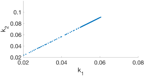
The time taken by our approach is quite competitive when compared to MCMC samples. However, the timing comparison is not representative since the number of samples for MCMC varies across benchmarks to achieve a given variance for our estimates of E(p). In general, larger benchmarks require more samples. However, some of the benchmarks are challenging even though the number of parameters is small. For instance, the two-parameter Dalla-Man model instance exhibits a strong correlation between the parameters as seen in Fig. 3. This poses a challenge for all the MC approaches as well as our approach.
5 Conclusion
We propose an approach to compute the approximation of the posterior distribution. In the proposed method, the parameter space is divided into multiple subsets, and the cells with the highest probability are refined through iterations. The proposed method calculates the probability bounds of the cells for computing the likelihood. This calculation is achieved by using a reachability analysis and bounding the value of the integration of likelihood. The approach is evaluated over several nonlinear benchmarks with a varying number of parameters and compared with MCMC samplers. The bounds of the posterior can also to be used to infer the probability bounds of satisfaction of properties. Future work will investigate approaches to factor the joint distribution over numerous parameters into simpler distributions over subsets of parameters by analyzing how they are correlated. This can help our approach scale to larger parameter spaces.
Acknowledgments
We are thankful to the anonymous reviewers and Prof. Nisar Ahmed for their valuable suggestions. This work was supported in part by the US National Science Foundation (NSF) under award number CCF 1815983 and the US Air Force Research Laboratory (AFRL). All opinions expressed are those of the authors and not necessarily of our sponsors.
@inproceedings{ijcai2019p791,
  title     = {Bayesian Parameter Estimation for Nonlinear Dynamics Using Sensitivity Analysis},
  author    = {Chou, Yi and Sankaranarayanan, Sriram},
  booktitle = {Proceedings of the Twenty-Eighth International Joint Conference on
               Artificial Intelligence, {IJCAI-19}},
  publisher = {International Joint Conferences on Artificial Intelligence Organization},
  editor    = {Sarit Kraus},
  pages     = {5708--5714},
  year      = {2019},
  month     = {8},
  note      = {Main track},
  doi       = {10.24963/ijcai.2019/791},
  url       = {https://doi.org/10.24963/ijcai.2019/791},
}
TY - CPAPER TI - Bayesian Parameter Estimation for Nonlinear Dynamics Using Sensitivity Analysis AU - Chou, Yi AU - Sankaranarayanan, Sriram T2 - Proceedings of the Twenty-Eighth International Joint Conference on Artificial Intelligence, IJCAI-19 PB - International Joint Conferences on Artificial Intelligence Organization PY - 2019 SP - 5708 EP - 5714 DO - 10.24963/ijcai.2019/791 UR - https://doi.org/10.24963/ijcai.2019/791 ER -Copied
Machine-readable versions of this paper, for tools and AI agents:





