
Finding Optimal Solutions in HTN Planning - A SAT-based Approach
Proceedings of the Twenty-Eighth International Joint Conference on Artificial Intelligence. Main track. Pages 5500-5508.
https://doi.org/10.24963/ijcai.2019/764
© 2019 International Joint Conferences on Artificial Intelligence
Keywords
- Planning and Scheduling: Planning Algorithms
- Planning and Scheduling: Hierarchical planning
- Constraints and SAT: SAT: Applications
Abstract
Over the last years, several new approaches to Hierarchical Task Network (HTN) planning have been proposed that increased the overall performance of HTN planners.
However, the focus has been on agile planning - on finding a solution as quickly as possible.
Little work has been done on finding optimal plans.
We show how the currently best-performing approach to HTN planning - the translation into propositional logic - can be utilised to find optimal plans.
Such SAT-based planners usually bound the HTN problem to a certain depth of decomposition and then translate the problem into a propositional formula.
To generate optimal plans, the length of the solution has to be bounded instead of the decomposition depth.
We show the relationship between these bounds and how it can be handled algorithmically.
Based on this, we propose an optimal SAT-based HTN planner and show that it performs favourably on a benchmark set.
- [Alford et al., 2016] Ron Alford, Gregor Behnke, Daniel Höller, Pascal Bercher, Susanne Biundo, and David W. Aha. Bound to plan: Exploiting classical heuristics via automatic translations of tail-recursive HTN problems. In ICAPS, pages 20-28, 2016.
- [Behnke et al., 2015] Gregor Behnke, Daniel Höller, and Su- sanne Biundo. On the complexity of HTN plan verification and its implications for plan recognition. In ICAPS, pages 25-33, 2015.
- [Behnke et al., 2017] Gregor Behnke, Daniel Höller, and Su- sanne Biundo. This is a solution! (... but is it though?) - Verifying solutions of hierarchical planning problems. In ICAPS, pages 20-28, 2017.
- [Behnke et al., 2018a] Gregor Behnke, Daniel Höller, and Susanne Biundo. totSAT -Totally-ordered hierarchical planning through SAT. In AAAI, pages 6110-6118, 2018.
- [Behnke et al., 2018b] Gregor Behnke, Daniel Höller, and Susanne Biundo. Tracking branches in trees -A propo- sitional encoding for solving partially-ordered HTN plan- ning problems. In ICTAI, pages 73-80, 2018.
- [Behnke et al., 2019a] Gregor Behnke, Daniel Höller, and Susanne Biundo. Bringing order to chaos -A compact representation of partial order in SAT-based HTN plan- ning. In AAAI, 2019.
- [Behnke et al., 2019b] Gregor Behnke, Marvin Schiller, Matthias Kraus, Pascal Bercher, Mario Schmautz, Michael Dorna, Michael Dambier, Wolfgang Minker, Birte Glimm, and Susanne Biundo. Alice in DIY-wonderland or: In- structing novice users on how to use tools in DIY projects. AI Communications, 32(1):31-57, 2019.
- [Bercher et al., 2014] Pascal Bercher, Shawn Keen, and Su- sanne Biundo. Hybrid planning heuristics based on task decomposition graphs. In SoCS, pages 35-43, 2014.
- [Bercher et al., 2017] Pascal Bercher, Gregor Behnke, Daniel Höller, and Susanne Biundo. An admissible HTN planning heuristic. In IJCAI, pages 480-488, 2017. IJCAI
- [Bercher et al., 2019] Pascal Bercher, Ron Alford, and Daniel Höller. A survey on hierarchical planning -One abstract idea, many concrete realizations. In IJCAI, 2019. IJCAI
- [Chowdhury et al., 2018] Md Solimul Chowdhury, Martin Müller, and Jia-Huai You. Description of expsat solvers. In SAT Comp. 2018, pages 22-23, 2018.
- [Erol et al., 1994] Kutluhan Erol, James Hendler, and Dana Nau. UMCP: A sound and complete procedure for hierar- chical task-network planning. In AIPS, 1994.
- [Erol et al., 1996] Kutluhan Erol, James Hendler, and Dana Nau. Complexity results for HTN planning. Annals of Mathematics and AI, 18(1):69-93, 1996.
- [Geier and Bercher, 2011] Thomas Geier and Pascal Bercher. On the decidability of HTN planning with task insertion. In IJCAI, pages 1955-1961, 2011. IJCAI
- [Gocht and Balyo, 2017] Stephan Gocht and Tomáš Balyo. Accelerating sat based planning with incremental sat solv- ing. In ICAPS, pages 135-139, 2017.
- [Helmert and Domshlak, 2009] Malte Helmert and Carmel Domshlak. Landmarks, critical paths and abstractions: What's the difference anyway? In ICAPS, 2009.
- [Höller et al., 2014] Daniel Höller, Gregor Behnke, Pascal Bercher, and Susanne Biundo. Language classification of hierarchical planning problems. In ECAI, 2014.
- [Höller et al., 2018] Daniel Höller, Pascal Bercher, Gregor Behnke, and Biundo Biundo. A generic method to guide HTN progression search with classical heuristics. In ICAPS, pages 114-122, 2018.
- [Höller et al., 2019] Daniel Höller, Pascal Bercher, Gregor Behnke, and Susanne Biundo. On guiding search in HTN planning with classical planning heuristics. In IJCAI, 2019. IJCAI
- [Nau et al., 1999] Dana Nau, Yue Cao, Amnon Lotem, and Hector Munoz-Avila. SHOP: Simple hierarchical ordered planner. In IJCAI, pages 968-973, 1999. IJCAI
- [Nau et al., 2003] Dana Nau, Tsz-Chiu Au, Okhtay Ilghami, Ugur Kuter, J. Murdock, Dan Wu, and Fusun Yaman. SHOP2: An HTN planning system. Journal of Artificial Intelligence Research (JAIR), 20:379-404, 2003.
- [Rintanen et al., 2006] Jussi Rintanen, Kejio Heljanko, and Ilkka Niemelä. Planning as satisfiability: parallel plans and algorithms for plan search. Artificial Intelligence, 170(12-13):1031-1080, 2006.
- [Ryvchin and Nadel, 2018] Vadim Ryvchin and Alexander Nadel. Maple LCM Dist ChronoBT: Featuring chrono- logical backtracking. In SAT Comp. 2018, page 29, 2018.
- [Schreiber et al., 2019] Dominik Schreiber, Tomáš Balyo, Damien Pellier, and Humbert Fiorino. Tree-REX: SAT- based tree exploration for efficient and high-quality HTN planning. In ICAPS, 2019.
- [Sinz, 2005] Carsten Sinz. Towards an optimal CNF encod- ing of boolean cardinality constraints. In CP, 2005.
- [Soos, 2018] Mate Soos. The CryptoMiniSat 5.5 set of solvers at the SAT competition 2018. In SAT Comp., 2018.
- [Sreedharan et al., 2018] Sarath Sreedharan, Tathagata Chakraborti, and Subbarao Kambhampati. Handling model uncertainty and multiplicity in explanations via model reconciliation. In ICAPS, pages 518-526, 2018.
- [Streeter and Smith, 2007] Matthew Streeter and Stephen Smith. Using decision procedures efficiently for optimiza- tion. In ICAPS, pages 312-319, 2007.
- [Torralba et al., 2016] Álvaro Torralba, Carlos Linares López, and Daniel Borrajo. Abstraction heuristics for symbolic bidirectional search. In IJCAI, 2016. IJCAI
- [Wilkins, 2000] David Wilkins. Using the SIPE-2 planning system -A manual for SIPE-2, version 6.1, 2000.
- [Xie et al., 2014] Fan Xie, Martin Müller, and Robert Holte. Jasper: The art of exploration in greedy best first search. In The 2014 IPC, pages 39-42, 2014.
References were extracted automatically from the PDF and may contain errors.
Full text extracted automatically from the PDF; figures, tables and equations may differ. The PDF is the version of record.
1 Introduction
In Hierarchical Task Network (HTN) planning [Bercher et al., 2019], a given abstract task has to be divided (decomposed) into other tasks until only tasks are left that can be executed directly. These tasks are identical to actions in classical planning. They are described by state-based preconditions and effects. The combination of a decomposition-based structure with state-based execution of actions forms a separate class of planning problems that can express much harder problems [Erol et al., 1996; H¨oller et al., 2014] than classical planning alone. This even includes un-decidable problems such as the Grammar Intersection Problem of Context-free Languages or Post's Correspondence Problem.
Several new approaches to solve HTN planning problems have been introduced over the last years and increased the overall performance of the systems in that field. These new techniques range from heuristic search in plan space [Bercher et al., 2017; Bercher et al., 2014], heuristic progression search [H¨oller et al., 2018; H¨oller et al., 2019], over the translation into classical planning problems [Alford et al., 2016], to translations into propositional logic [Behnke et al., 2019a; Behnke et al., 2018b; Behnke et al., 2018a; Schreiber et al.,
2019]. Both translation-based approaches bound the original problem to be able to translate the undecidable HTN planning problem into a decidable one. Currently, the SAT-based approach shows the best performance. It bounds the planning problem to a certain decomposition depth and translates the resulting problem into a propositional formula.
In many practical settings, it is not only important to find a plan that reaches a given goal, but to find an optimal one. For example in transport and delivery domains, optimality is desired to save costs. Especially when interacting with human users optimality is often required. Non-optimal plans will often contain additional actions that humans can easily spot as superfluous, which is problematic when the generated plan is used to assist or instruct humans [Behnke et al., 2019b]. For plan explanations in the form of model reconciliation, optimal plans are necessary as well [Sreedharan et al., 2018].
Despite progress in HTN planning, little work has been done to find optimal plans. Only one system [Bercher et al., 2017] is able to find such plans, while H¨oller et al. [2018] proposed an admissible heuristic, but did not experiment with it. Optimal search-based HTN planners face a problem not present in classical forward search (though known from Partial Order Causal Link planning): Due to the decompositions performed during search, the goal distance in the search space is not equal to the length of the solution, as the latter only contains actions. To find length-optimal plans, an admissible heuristic has to estimate the length of the plan and not the distance in the search space, leading to poor search guidance.
We introduce the first SAT-based approach for optimal HTN planning. In it, the length of the solution has to be bounded instead of the decomposition depth. We have previously preposed techniques for computing such bounds in the context of HTN plan verification Behnke et al. [2017]. In this paper, we show that our previous bounds were unnecessarily high. The new bound computation improves them by up to three magnitudes. Our new depth bound computation can even show that no plan of a given length can exist, which was not recognised by previous methods. We discuss three different algorithms to find optimal solutions with the new bounding method. We compare our new planner against the optimal planner from the literature [Bercher et al., 2017], a progression-based planner with an admissible heuristic [H¨oller et al., 2018], and modify the planner by Alford et al. [2016] to find optimal solutions.
2 HTN Planning
In this section we introduce the HTN formalism by Geier and Bercher [2011] that is used throughout the paper. In HTN planning, two types of tasks are distinguished: primitive tasks (also called actions) and abstract tasks. Let P and C be the set of primitive and abstract tasks. Abstract tasks represent courses of action that can not be executed directly. They need to be divided into more concrete tasks until executable tasks are reached. These are the primitive tasks. World states are described using a set of propositional state variables V . Each primitive task is associated with a set of preconditions pre(p) ⊆ V that need to hold for it to be applicable and effects del (p), add(p) ⊆ V defining state variables that are deleted and added when the action is applied. Tasks are organised in task networks, partially ordered sets of tasks. Formally a task network is a triple (I,≺, α) where I is a - potentially empty - set of IDs, ≺ is a partial order on I, and α : I → P ∪ C labels each ID with a task. Using IDs is necessary as a task network might contain the same task twice.
The objective in HTN planning is given in terms of a single abstract task AI - the initial task. A solution to the problem is a decomposition of AI into actions that are executable in the initial state s0. A task t is decomposed by replacing it with the contents of one of its applicable methods. A method is a pair (A, tn) where A is an abstract task and tn a task network. Formally, we always decompose a task within a task network and start the process with the task network tnI = ({l1}, ∅, {(l1,AI)}), i.e. one containing only the initial task. The application of decomposition methods is akin to applying derivation rules in formal grammars - with the difference that we don't handle sequences of tasks, but partially-ordered sets.
Definition 1. Let tn = (I,≺, α) be a task network, i ∈ I an ID with α(i) = A with A ∈ C and m = (A, (Im, ≺m, αm)) with Im ∩ I = ∅ a decomposition method. Decomposing i in tn using the method m results in the task network tn′ = (I ′ ,≺′ , α′ ) = D(tn, i,m) with I ′ = (I ∪ Im) \ {i}, α′ = (α ∪ αm) \ {(i, A)}, and ≺′= (≺ ∪ ≺m ∪ ≺I ) ∩ (I ′ × I ′ ) where ≺I is the set of ordering constraints relative to i that are inherited to the newly added tasks, i.e.
Let D(tn) be the set of all decompositions of a task network tn and D∗ the transitive closure of D, i.e. tn′ ∈ D∗ (tn) iff tn′ can be obtained from tn via a sequence of decompositions.
Let M be the set of all methods. Many HTN planners allow for specifying method preconditions. A method with such a precondition can only be used if its precondition is fulfilled in some state before the first action resulting from it is executed, but after all actions preceding this task in the final task networks partial order are. Commonly, a method precondition prec is compiled into an additional action aprec whose precondition is prec and which does not have effects. This action precedes all other tasks in that method [Nau et al., 2003].
Definition 2. A solution to an HTN planning problem P = (V, P,C,M, s0,AI) is a sequence of actions π ∈ P ∗ that is executable in s0 such that there exists a task network tn ∈ D∗ (tnI) and π is a linearisation of the tasks in tn.
A sequence of applied decomposition methods leading from the task network containing the initial task AI to a task network tn is called tn's decomposition. A practically important structural measure for the complexity of this decomposition is its depth. Intuitively, the depth of a decomposition is the maximum number of methods that have to be applied to tasks in order to create the tasks contained in tn out of them. Formally, consider a decomposition of AI into a task network tn, which consists of a sequence of task networks tnI = tn1, . . . , tnn = tn such that tni ∈ D(tni-1). The decomposition depth d(j, tni) of a task ID j in any task network tni is defined as: (1) d(j, tnI) = 0 if i is contained in tnI, (2) d(j, tni) = d(j, tni-1) if j was not decomposed in tni-1, and (3) d(j, tni) = 1 + d(k, tni-1) if k was decomposed in tni-1 and k was inserted into tni via this decomposition. The decomposition depth of tn under the given decomposition is then the maximum decomposition depth of any task in tn. Another way to describe the decomposition depth is the following. Any decomposition can be viewed as a tree - the Decomposition Tree [Geier and Bercher, 2011] whose nodes are all the task IDs occurring during decomposition. Edges connect two IDs i and j if the decomposition of i inserted j into a task network. The decomposition depth is then the maximum depth of the Decomposition Tree.
Several methods have been proposed to solve HTN planning problems. Next, we briefly review these techniques.
Plan-space search. The first HTN planning systems, like SIPE [Wilkins, 2000] and UMCP [Erol et al., 1994], used plan-space search. In addition UMCP used simple heuristics to speed-up the search. Even in its Breath-First-Search configuration UMCP was not optimal in the sense that it produced the shortest plan. Instead it found the solution with the smallest number of modifications required. PANDA [Bercher et al., 2017] uses plan-space search in combination with the admissible TDG heuristic, which comes in two variants TDG-m and TDG-c. The former estimates the number of modifications needed to turn the current plan into a solution, while the latter estimates the number of additional actions that will be present in a solution. PANDA with A∗ search and the TDG-c heuristic constitutes the - to the best of our knowledge - first length-optimal HTN planner.
Progression search. Next to plan-space search, early HTN planners also used progression-based algorithms, e.g. SHOP and SHOP2 [Nau et al., 1999; Nau et al., 2003]. These planners generally used some form of depth-first search, which is not optimal with respect to the plan length. Recently, H¨oller et al. [2018] introduced an improved progression algorithm and a means to transform any heuristic for classical planning into one for HTN progression search. This is done via encoding a relaxed version of the HTN problem into a classical planning problem and subsequently applying a classical heuristic to it. The translation is admissible in the sense that if an admissible classical heuristic is applied to the encoded model, its estimate will be admissible for the HTN planning problem [H¨oller et al., 2018]. The translation evaluated in the paper is only admissible with respect to number of modifications, as costs are associated with both actions and methods.
Transformation into classical planning. Since HTN planning is undecidable [Erol et al., 1996], there can be no translation of HTN planning problems into other decidable problems. However, it is possible to bound the problem and to translate the bounded problem into another decidable problem, like classical planning. To achieve completeness, one needs to increment this bound until a solution has been found. Alford et al. [2016] proposed a translation that simulates a progression search in a classical planning problem. The encoding bounds the number of tasks in intermediate task networks - called the progression bound. Bercher et al. [2017] used this translation as a comparison for their optimal planspace planner PANDA. They used the optimal classical planner SymBA∗ [Torralba et al., 2016] to solve the classical planning problems. At this time we assumed that such a combination is optimal for the HTN planning problem - although this is not explicitly stated in the paper. This assumption was however incorrect. Consider an HTN planning problem with the abstract tasks A,B,C,D,X, Y ,Z where AI = A and primitive tasks a, b, c, d. The decomposition methods are: A → aB1 , B → bC, C → cD, D → d, A → XYZ, X → a, Y → b, Z → c. For progression bound 2, the only possible plan is abcd of length 4 using the first four methods. For progression bound 3, the plan abc of length 3 can be derived through the last four methods. Consequently, simply using an optimal classical planner does not yield an optimal HTN planner.
Transformation into propositional logic We recently proposed a translation of HTN problems into propositional logic, bounding the decomposition depth of the problem [Behnke et al., 2018a; Behnke et al., 2018b; Behnke et al., 2019a]. We construct a formula for a given HTN planning problem P and a depth bound K that is satisfiable if and only if P has a solution with a decomposition depth ≤ K. As this formula represents exactly all plans with decompositions depth ≤ K, it accounts for plans up to the maximum length achievable by decompositions of depth ≤ K. While heuristic searchbased techniques have to consider the interaction between constraints imposed via the actions' state-transition semantics and the decompositional structure of the problem explicitly, a SAT-based approach translates the whole problem into a single homogeneous representation. This allows SAT solvers to reason about the whole problem, making it a promising candidate for an efficient planner.
3 Optimal SAT-based HTN Planning
To test whether a given plan of length ℓ is optimal, we have to show that there is no plan of length ≤ ℓ-1. For a SAT-based planner, this means to construct a propositional formula that is satisfiable if and only if there is a solution of length ≤ ℓ-1. In SAT-based classical planning, this is (somewhat) trivial as formulae are constructed based on a plan-length bounded problem 2 . The propositional encoding for HTN planning limits the decomposition depth instead. Given a depth limit K, we can easily derive a length limit ℓ(K) by extracting the longest reachable plan via decomposition up to that depth. This limit does not conversely imply that all plans of length ℓ(K) have a depth of at most K, but only that plans longer than ℓ(K) have a depth of at least ℓ(K)+1. As a counter example, consider an HTN planning problem with the abstract tasks A and B and three actions a, b, and c. Let there be three methods: A → abc, A → aB, and B → b. For the depth limit K = 1 the length bound ℓ(K) is 3, but it is not possible to represent the plan ab of length two with that depth bound.
1A → ω denotes a method decomposing A into a task network containing the tasks ω as a sequence.
2 The construction becomes more complicated if we use an encoding allowing for parallelism, like ∃-step [Rintanen et al., 2006].
For optimal planning, we have to determine a depth bound K(ℓ) such that all decompositions leading to any plan of length ≤ ℓ have a decomposition depth of at most K(ℓ).
Definition 3 (Maximum Decomposition Depth - Preliminary Definition). Let P be an HTN planning problem and ℓ be an integer. K(ℓ) is the minimum depth such that all decomposition trees with at most ℓ leafs have a depth of at most K(ℓ).
This definition could be modified to ask for the minimum depth such that all decomposition trees whose leafs can be executed (i.e. those representing solutions) with at most ℓ leafs have a depth of at most K(ℓ). Even approximating this bound is however quite complicated. We instead focus on the given definition, which is an upper bound for the stricter one.
Unfortunately, the value of the depth bound in this definition might be infinite for some HTN planning problems. This is caused by specific structures occurring in a problem's decompositions. We will describe and tackle those issues later on in the paper (Sec. 3.2). For the time being, we will discuss computing K(ℓ) only for HTN planning problems with the following restrictions:
- All decomposition methods contain at least one subtask.
- If a decomposition method contains only a single subtask, it is primitive.
These restrictions are a sufficient condition ensuring that K(ℓ) - as defined in Def. 3 - is finite. We will start by describing an algorithm that computes K(ℓ). Thereafter, we will show how K(ℓ) can be defined for problems containing the two types of excluded methods. Lastly, we will extend the base algorithm so that it can compute K(ℓ) in general, i.e. unrestricted, planning problems.
3.1 Computing K for Benign Problems
We have previously (in the context of HTN plan verification) proposed three different methods to compute approximations for the depth bound K(ℓ) based on a given plan length ℓ. Of them, one can always use the minimum of them [Behnke et al., 2017]. We will briefly describe these methods.
K1: The first method is based on a theoretical result 3 from HTN plan verification [Behnke et al., 2015]. Their approximation of the bound is solely based on the considered plan length ℓ and the number of abstract tasks |C|. It is defined as K1(ℓ) = 2 · (ℓ-1) · (|C| +1). Its value is often far too high. K2: The second method is based on the Task Schema Transition Graph (TSTG) [Behnke et al., 2017]. A TSTG T describes an abstraction to the possible decompositions in an
3 Note that the lemma in the paper erroneously states a bound that is half the size of the bound given here.
Algorithm 1 Calculate K4(ℓ) - base algorithm
global K(A, ℓ) =∞ function compute K4(ℓmax ) compute SCCs S of the problem's TSTG for SCC S ∈ S in reverse topological order do if |S| = 1 and for p ∈ S holds that p ∈ P then K(p, 1) = 0 else for ℓ = 1 to ℓmax do updateSCC(ℓ, S) end for end if end for function updateSCC(ℓ, S) for A ∈ S and m = (A, (I, ≺, α)) ∈ M do for φ : I → N with ∑i∈I φ(i) = ℓ do K∗ = 1 + maxi∈I K(α(i), φ(i)) K(A, ℓ) = max{K(A, ℓ), K∗ } end for end forHTN planning problem. T's vertices are the abstract tasks. There is a directed edge A → B between two vertices A and B iff there is a method decomposing A that contains B in its task network [Behnke et al., 2017]. If the TSTG T is acyclic 4 , the length of its longest path is a bound to the depth of any possible decomposition tree [Behnke et al., 2017].
K3: The last method is only applicable to HTN planning problems in which every decomposition method has at least two subtasks. In them, the size of the current task network grows with each decomposition by at least one. Let δ be the minimum number of subtasks in any method. Then, K3(ℓ) = ℓ δ-1 is an upper bound [Behnke et al., 2017].
Only method K1 is applicable to arbitrary planning problems, which however tends to compute overly high bounds (see Sec. 5). K2 and K3 require additional structure in the planning problem to be applicable. We will show in our evaluation that the bounds computed with these three methods are far too high. A propositional encoding based on these bounds could not be constructed in practice. Thus all three methods are not well suited to optimal planning.
We propose a new method to compute the bound K4, which (1) strictly dominates all the other methods and (2) leads to significantly smaller bounds. It is described in terms of pseudo-code in Alg. 1. We start the description of our algorithm with the assumption of a restricted HTN planning problem, namely one fulfilling the two conditions stated above.
Our method is based on computing an individual bound K4(A, ℓ) for each abstract task A and plan length ℓ. As a generalisation of K(ℓ), K4(A, ℓ) shall be the maximum decomposition depth starting from A (and not specifically AI) into a task network containing exactly ℓ primitive actions. Since K4(A, ℓ) accounts only for the decompositions into exactly ℓ primitive actions, we return K4(ℓ) = mink≤ℓ K4(AI , k).
Definition 4. Let P be an HTN planning problem, ℓ an integer, and A ∈ P ∪ C a task. K4(A, ℓ) is the minimum depth such that all decomposition trees with at most ℓ leafs whose root task is A have a depth of at most K(ℓ).
4 This is equivalent with the planning problem being acyclic.
Trivially K4(p, ℓ) = 0 for any primitive task p if ℓ = 1 and -∞, else. The latter represents that it is impossible to decompose primitive tasks.
To compute K4(A, ℓ), we process the abstract tasks A "up the hierarchy". For this, we use the TSTG T, which represents a relaxed version of the problem's decomposition hierarchy. Note that the value of K4(A, ℓ) for an abstract task A depends only on the values of K4(B, ℓ) of all its direct successors in T. This is due to the fact that a decomposition tree starting at A must apply some method applicable to A which can only result in tasks which are successors of A in T (and potentially further primitive actions). If the TSTG T is acyclic, we can compute K4(A, ℓ) for the abstract tasks in reverse topological order - as the value K4(A, ℓ) depends only on the successors B - for which the values K(B, ·) have already been computed.
Unfortunately, HTN planning problems do not always have an acyclic TSTG. If T contains cycles, we process its Strongly Connected Components (SCCs) in reverse topological order. As for acyclic TSTGs, whenever we process a SCC S of T , the K4(A, ℓ) values for all tasks occurring in methods for tasks in S have already been computed - except for those that are members of S. Thus we have to compute the values of K4(A, ℓ) for a single SCC S at a time.
To do so, we propose an iterative algorithm, which iterates over the depth of the considered decompositions. In each iteration, we consider the decompositions of every A starting with a method m = (A, tn = (I , ≺, α)) applicable to it anew. For each subtask B in tn we either know its correct K4(B, ℓ) values (if B ̸∈ S) or a current estimate (if B ∈ S). We can then try to obtain a new lower bound K∗ for the value of K4(A, ℓ). In this decomposition, we first apply m and then continue with decompositions of depth ≤ K∗ - 1 for each of the tasks in tn, where at least one decomposition has the depth K∗ - 1. These decompositions together must produce ℓ actions, i.e. a (potential) plan of length ℓ. Each of the tasks (identifiers) i in tn will be decomposed into a number of primitive actions, which we will denote with φ(i). These decompositions lead to ℓ actions in total if ∑i∈I φ(i) = ℓ. Note that φ(i) has to be at least 1 for every subtask, as there are no empty decomposition methods in the planning problem. Consequently K4(A, 0) will always be infinity.
Given such a distribution φ of primitive actions to subtasks on m, we can compute a new lower bound K∗ for K4(A, ℓ). The currently known maximum decomposition depth for each subtask i and associated length φ(i) can be retrieved via a table lookup. K∗ is then 1+maxi∈I K4(α(i), φ(i)). This composition of length bounds is depicted in Fig. 1. As we have found a new decomposition of A, we can update K4(A, ℓ) to the maximum of its old value and the just computed K∗ , i.e. we can set K4(A, ℓ) = max{K∗ ,K4(A, ℓ)}. To obtain completeness, we have to consider all possible distributions φ such that ∑i∈I φ(i) = ℓ. Since explicitly enumerating all these distributions is impossible, we use dynamic programming to speed-up the computation.
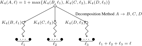
To fully compute the K4(A, ℓ) values, we iterate the update ℓ times. Initially, we set all the K4(A, ℓ) for A ∈ S to -∞.
Lemma 1. After the j th iteration, we have computed the entries K4(A, ℓ) for ℓ ≤ j correctly.
Proof. This can be shown via induction. For plan length ℓ = 1, any decomposition method must not contain tasks in S, else we have to assign zero primitive tasks to any task in S Thus the values for K4(A, 1) are computed correct after one update. At the j th iteration with j ≥ 2, consider the decomposition with maximum depth of a task A into j primitive tasks. This decomposition starts with a method m = (A, tn) and assigns φ(i) primitive tasks to each of the subtasks of tn. tn must contain at least two subtasks (else the single subtask must be primitive which is incompatible with having j ≥ 2 primitive tasks after all decompositions). Next, φ can assign at most ℓ-1 primitive tasks to any task in S, else there would be some subtask assigned zero primitives, which is not possible. By induction all K4(i, φ(i)) have already been computed correctly, making the computed value K4(A, ℓ) correct.
3.2 Handling Empty Cycles
So far, the algorithm has been designed for HTN planning problems without methods that decompose an abstract task into either an empty task network or a task network containing only a single abstract task. Such decomposition methods do, however, occur frequently in HTN planning problems. Further, handling them allows our bound computation method K4 to cover all HTN planning problems - without requiring any additional structure in it.
The reason for excluding the mentioned types of methods is that their presence allows for a structure in decompositions that we call an empty cycle. An empty cycle is a non-empty sequence of decompositions for an abstract task A resulting in a task network containing only the abstract task A. I.e. we can apply a sequence of decompositions that does not change the task network. These empty cycles allow for arbitrarily deep decompositions resulting in the same task network. As an example, consider the three methods decomposing A into B and C, B into A, and C into an empty task network. One might consider removing these cycles from the HTN planning problem, as they do not contribute any relevant structure; but the individual decompositions might still be necessary. We might e.g. have to apply the method decomposing A into B and C and then decompose C into a and B into b. Another idea would be to replace sets of abstract tasks S that can be transformed into each other via empty cycles by a single new abstract task. This would remove the need for methods that are part of empty cycles allowing to remove them. This is also incorrect since decomposition methods inside the cycle might be associated with method preconditions - and thus we have to track how the transformation between these "equivalent" tasks takes place. They do not add new tasks to a task network, but impose constraints for decompositions. Simply ignoring them via this construction would remove the constraints posed by them.
Thus, we have to explicitly consider the methods that may lead to empty cycles in a planning problem. As a result, the depth bound definition given above (Def. 3) is not usably any more: If the planning problem allows for empty cycles K(ℓ) (as defined before) would be infinity. As a consequence, we have to adapt the definition explicitly considering only depths of those decomposition trees that do not contain empty cycles.
Definition 5 (Maximum Decomposition Depth - Final Definition). Let P be an HTN planning problem and ℓ be an integer. K(ℓ) is the minimum depth such that all decomposition trees T with at most ℓ leafs have a depth of at most K(ℓ), such that there are no two nodes t1, t2 in T where:
- α(t1) = α(t2) and
- t2 is an (indirect) successor of t1 in T and
- the decompositions between t1 and t2 could be removed, including t2, without altering the yield of T, i.e. the decompositions between t1 and t2 form an empty cycle.
Intuitively spoken K4 is - for a given length bound ℓ - the maximum decomposition depth K(ℓ - 1) such that all plans of length ≤ ℓ - 1 have a decomposition depth of at most K(ℓ - 1), excluding those that contain empty cycles. Note that we will retain completeness as whenever we exclude a decomposition because it contains an empty cycle, there will be a decomposition for the same plan with equal or lower depth that does not contain that empty cycle. Removing these decompositions will also remove their method preconditions. Since removing them only loosens restrictions, but does not alter or add any other restriction, we preserve any solution, i.e. executable linearisation of leafs.
As did the previous algorithm for restricted domains planning problems, we will not compute K(ℓ) directly, but we will compute a depth bound K4(A, ℓ) for every abstract task A. Further, we do not aim at computing these values exactly. Instead we aim only at computing an approximation of the actual value of K4(A, ℓ), i.e. a value that is not lower than the correct value. The proposed algorithm is shown in Alg. 2.
As a basis, we re-use the algorithm described in the previous section: Treat the SCCs S of the TSTG in reverse topological order and update the estimates for K4(A, ℓ) inside each component iteratively. This is done via considering every applicable decomposition method and distributing the ℓ primitive tasks to produce between the subtasks of the method. If the problem - as was the case in the previous section - does not contain any method with empty task network, at least one primitive task must be assigned to every subtask, as it is not possible to decompose any task into a solely primitive task network containing less than one primitive task. In the general case we are considering now, assigning plan length zero to an (abstract) subtask of a method is in
Algorithm 2 Calculate K4(ℓ)
global K(A, ℓ) =∞ function compute K4(ℓmax ) compute SCCs S of the problem's TSTG for SCC S ∈ S in reverse topological order do if |S| = 1 and for p ∈ S: p ∈ P then K(p, 1) = 0 else computeSCC(ℓmax , S) end if end for function computeSCC(ℓmax , S) for round1 = 1 to |S| + 1 do updateSCC(ℓmax , S, false) for round2 = 1 to |S| - 1 do updateSCC(ℓmax , S, true) end for end for function updateSCC(ℓmax , S, considerEmpty) for ℓ = 0 to ℓmax do for A ∈ S and m = (A, tn = (I, ≺, α)) ∈ M do for do for φ : I → N with ∑i∈I φ(i) = ℓ do ε-decomposition := ∃i∗∈I:α(i∗ ) ∈ S and ∀i∈I\{i∗ }:φ(i)=0 if considerEmpty ̸= ε-decomposition then continue end if K∗ = 1 + maxi∈I K(α(i), φ(i)) K(A, ℓ) = max{K(A, ℓ), K∗ } end for end for end for end forprinciple possible. Such assignments would allow for empty cycles. Specifically, an empty cycle contains decompositions where φ assigns the whole plan length ℓ to a single task i∗ in tn that is a member of S and 0 to all other subtasks. Since we only want to consider decompositions without empty cycles, we exclude such assignments from the computation of the base algorithm. Apart from this exclusion, we start by applying the updateSCC function in an unaltered form.
When running the (modified) base algorithm, we exclude methods containing only a single abstract task that is contained in S and assignments φ that assign the whole plan length ℓ to an abstract task in S. We will call these decompositions ε-type decompositions, as they could lead to an empty cycle. When computing the depth bound K4(A, ℓ) we cannot exclude these methods fully, as they can e.g. provide the only means to obtain a primitive plan. To integrate them, we use the same update-mechanism as we did in the first step of the algorithm. Instead of considering all non-ε-type decompositions, we will here consider only such decompositions. We iterate until any further iteration will solely account for decompositions containing empty cycles. This is the case if we have executed the computation |S| - 1 times.
Lemma 2. After |S| - 1 iterations with ε-type decomposition, every additional update only accounts for decompositions containing empty cycles.
Proof. Consider the |S|th iteration of the computation and assume that there is a non-cyclic decomposition that is new to consideration at this step. Let m be the first applied method and A the respective abstract task. Consider the path in the decomposition that, starting from the root A decomposes only tasks in S. Since this decomposition was new to consideration after |S| steps, this path starts with |S| ε-type decompositions, else it would have been considered in a previous step. As it contains |S| steps, i.e. individual applications of decompositions of the ε-type, the path contains |S|+1 abstract tasks from S, i.e. at least one twice. Since we only considered εtype methods, this constitutes an empty cycle.
If we have executed the second step of the algorithm, we have still excluded some decompositions from consideration. This is the case if we, e.g. first apply decompositions of the ε-type, then one non-ε decomposition and then again ε-type decompositions. An example would be a problem with the abstract tasks A, B, C, D and methods A → B (1), B → C (2), C → D (3), D → A (4), C → Da (5), and B → b (6). In order to obtain a plan of length two from A we would have to use the following decomposition methods: (1), (2), (5), (4), (1), (6). Applying steps one and two of the algorithm accounts only for decompositions, which - viewed from the root task - first use only ε-type methods and then methods of non-ε type and subsequently leave S. To consider any interleaving of ε and non-ε methods we repeat steps one and two of the algorithm. We have to iterate these two steps until we are sure that only decompositions containing an empty cycle are newly considered by the iteration. This is the case after |S| + 1 iterations. Each application of a method of nonε type decreases the number of actions to be produced by the abstract task remaining in the SCC by one. I.e. we can only apply |S| such methods where the last one might assign length 0 to a task in the SCC. To consider this case, we need an additional round of the algorithm.
3.3 The Overall System
For the overall planner, we can use the same iteration technique as in classical planning: start with length bound ℓ = 1 and increase by one if no plan exists. For each length bound ℓ, we compute the depth bound K(ℓ) and construct the propositional formula used for non-optimal planning [Behnke et al., 2019a]. The formula however also permits solutions that contain more actions than the current length bound. As such, we have to bound the number of actions in the plan represented by a valuation of the formula. In the formula, the plan is represented as a sequence of timesteps. For each timestep t and for each action a there is an atom a@t representing that action a is executed at time t. Note that, since the encoding uses the ∃-step encoding [Rintanen et al., 2006] for primitive executability, more than one a@t atom can be true for every timestep. To restrict the plan to a length of at most ℓ actions, we have to ensure that at most ℓ of the a@t atoms are true. This type of constraint is common in propositional encodings, so compact and efficient encodings are readily available. We use the sequential encoding [Sinz, 2005]. As we have noted in Sec. 2, HTN planning problems often also include method preconditions, which are translated into additional actions in the model. These actions do not contribute to the length of the plan as they are artificial helper actions. We can account for this by not considering them for the at-most-ℓ restriction.
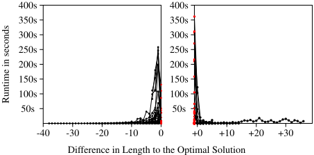
For classical planning, this simple incrementing strategy has already shown significant drawbacks. We will call this strategy INC(rement). It is identical to the strategy S of Rintanen et al. [2006]. The issue with it is that if the optimal solution has length L, the planner will test for all ℓ ≤ L whether a plan of length ℓ exists. Theoretically, it is only necessary to test L and L - 1, thus INC/S perform far to many checks. Furthermore, the runs for lengths ℓ slightly lower than L are generally difficult for SAT solvers (see Fig. 4).
Therefore several strategies have been developed to improve the performance of the overall algorithm. Rintanen et al. [2006] proposed the strategies A, B, and C, which parallelise the calls for different lengths ℓ. These strategies are primarily designed for satisficing, i.e. non-optimal, planning and abort the search process as soon as a first solution is found. They do not address the issue of determining the optimal solution. Gocht and Balyo [2017] and Schreiber et al. [2019] proposed to use an incremental SAT solver to use the search performed for ℓ to speed up the search for ℓ +1. We have not yet integrated our encoding with an incremental SAT solver, thus we have not considered such speed-ups. Streeter and Smith [2007] present bound-iteration strategies for optimal planning. They consider both the order in which bounds are tested as well as the time-limit for these tests. Their overall goal is not to find guaranteed optimal plans, but to narrow the interval in which an optimal plan lies as much as possible, explaining why they consider time-limits for individual runs. For simplicity, we do not consider such time-limits.
In addition to INC, we have tested two strategies: DEC(recment) and BIN(ary). BIN is - if we assume a time-limit of ∞ identical to the strategy S2 of Streeter and Smith [2007]. We start by running the planner in non-optimal mode to find any solution as quickly as possible. Once a solution has been found, its length ℓ∗ is an upper bound for the length of the optimal plan. For this non-optimal run, we use the incrementing strategy. We could speed it up further using any of the strategies by Rintanen et al. [2006], but have not done so. If the planner has found the first solution of length ℓ∗ at depth K∗ , we know that there is no solution with depth K∗ -1 or lower. Thus we can choose the highest length ℓ- as the lower bound such that K(ℓ-) ≤ K∗ - 1. We use binary search to find the length of the optimal solution between the upper and lower bounds and hence call the strategy BIN(ary).
Lastly, DEC starts off identical to BIN, but does not use binary search to find the optimal answer. Instead it simply decrements the upper bound on the plan length by one until no solution is found any more.
4 Making Other Systems Optimal
To ensure a fair competition against the state of the art in HTN planning, we considered how two approaches for HTN planning can be used to find optimal solutions.
Progression-based Planning
To make the progression-based approach by H¨oller et al. [2018] optimal, we have to make three changes: (1) use an A∗ search where the current path cost is the number of progressed actions, (2) set the costs of method actions in the heuristic model to zero, and (3) use an admissible classical heuristic to compute the heuristic value on the model. We use LM-Cut [Helmert and Domshlak, 2009] and denote the planner with "Progr. LM-Cut".
Translation into Classical Planning
The approach of Alford et al. [2016] suffers from the same problem as the SAT-based planner: its translations do not restrict the plan length but another measure, in this case the progression bound. As shown in Sec. 2 it is possible to find shorter solutions with a higher progression bound. For tailrecursive planning problems, we know that an upper limit P + to their progression bound exists, meaning that no plan requires a larger progression bound [Alford et al., 2016]. If so, we can use the translation with the bound P + and solve the resulting problem with an optimal classical planner. We used SymBA∗ , winner of the IPC 2014 and still one of the best optimal classical planners [Torralba et al., 2016]. We denote this planner with "HTN2STRIPS maxPB". This method leads to a very poor performance due to high maximum progression bounds in may instances. For most instances with high progression bounds, the planner cannot complete grounding within the time-limit.
We propose to use a technique similar to that for the SAT-based planner. We first run the encoding of Alford et al. [2016] in satisficing mode (with jasper [Xie et al., 2014]) to find an upper bound ℓ to the length of an optimal solution. We then compute the depth-bound K(ℓ - 1) required for any shorter plan. Next, we modify the HTN planning problem such that it is acyclic with a maximum decomposition depth of K(ℓ - 1) by replacing every abstract task A with tasks Ad for d ∈ [1,K(ℓ - 1)] and change the methods accordingly. This new problem is acyclic and thus has a finite progression bound P [Alford et al., 2016]. Any solution to the original encoding with a decomposition depth of at most K(ℓ - 1) will have a progression bound of at most P . We then run the translation on with original, i.e. non-altered model, the bound P and SymBA∗ . We don't use the compiled acyclic planning problem as in it every abstract task is duplicated K(ℓ - 1) times - which would thus lead to significant performance decreases for the classical planner. This new bound is smaller than P + and exists even for non-tail-recursive problems. We denote this planner with "HTN2STRIPS bounded maxPB".
5 Evaluation
We implemented the given techniques within the PANDA planning framework using its implementation of a propositional encoding for HTN planning [Behnke et al., 2019a; Behnke et al., 2018b; Behnke et al., 2018a]. The code can be downloaded at https://www.uni-ulm.de/en/in/ki/panda/.
We use the 144 instances from the most recent evaluations of satisficing HTN planners [Behnke et al., 2019a; H¨oller et al., 2018]. HTN2STRIPS max PB was only run on the 109 tail-recursive instances, as it can only find optimal solution on them. Each planner was given 10 minutes of runtime and 4 GB of RAM on an Intel E5-2660. For the propositional encoding, we used three SAT solvers: cryptominisat (cms) 5.5 [Soos, 2018], expMV [Chowdhury et al., 2018], and MapleLCM [Ryvchin and Nadel, 2018], some of the best performing SAT solvers in the 2018 SAT race.
Results
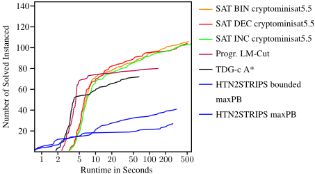
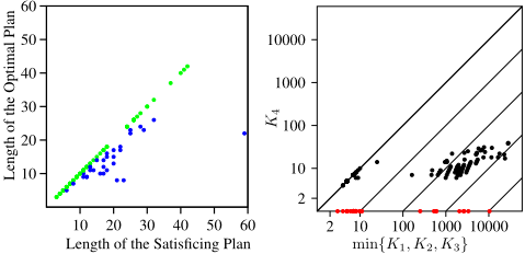
The number of optimally solved planning problems for each planner is shown in Tab. 1. The runtime behaviour is shown in Fig. 2. Both the SAT-based techniques described in this paper and progression search with the LM-Cut heuristic outperform the previously only existing optimal HTN planner PANDA. The SAT-based techniques solve between 19 and 26 more instances than the progression-based planner. Solely HTN2STRIPS lacks behind severely in performance, although our modifications improved its coverage. There is no pronounced difference between the algorithms INC, DEC, and BIN. INC and DEC are on par, while BIN solves ≈ 2 additional instances. We can see a significant difference between domains. INC is better in ROVER, while DEC and BIN perform better in TRANSPORT. Fig. 3 a) shows for DEC the relation between the length of satisficing and optimal solutions. The difference between INC and DEC on ROVER is caused by the quality of the initial non-optimal solution. The non-bounded SAT-encoding tends to produce longer plans on ROVER, resulting in additional calls for DEC. For the instance with the longest known optimal plan, the optimal solution has length 19, but the non-optimal planner's plan had length 43. This also causes the improvement for BIN - it required fewer futile runs. The converse is true for TRANSPORT, where nonoptimal solutions tend to be almost optimal.
In Fig. 3 b), we show a comparison between the three older methods to compute depth bounds K1, K2, and K3 and our new K4. While never being worse, K4 computes far lower depth bounds - up to three magnitudes lower. There were 37 cases (red dots), where the old methods computed a depth bound, while K4 returned -∞, i.e. showing that no plan of length ≤ ℓ can be derived via decomposition. For DEC, this led to instances in which we could show that the satisficing plan was already optimal. This is the case if for a satisficing plan of length ℓ, K4(ℓ - 1) is -∞. For SAT-DEC with cryptominisat 5.5, there were 34 such instances (19 UMTRANSLOG, 6 WOODWORKING, 1 SMARTPHONE, 2 PCP, 6 TRANSPORT). In Fig. 4, we show the time needed to solve each individual propositional formula in the INC and DEC strategies relative to the optimal plan length. We can clearly see that unsolvable instances near to the optimal solution are the most difficult formulae motivating the BIN strategy.
Acknowledgments
This work was done within the technology transfer project "Do it yourself, but not alone: Companion-Technology for DIY support" of the Transregional Collaborative Research Centre SFB/TRR 62 "Companion-Technology for Cognitive Technical Systems" funded by the German Research Foundation (DFG). The industrial project partner is the Corporate Research Sector of the Robert Bosch GmbH.
| SAT BIN | SAT DEC | SAT INC | HTN2 STRIPS | |||||||||
|---|---|---|---|---|---|---|---|---|---|---|---|---|
| #instances | cms 5.5 | expMV | MapleLCM | cms 5.5 | expMV | MapleLCM | cms 5.5 | expMV MapleLCM | Progr. LM-Cut TDG-c A* | bounded | maxPB maxPB | |
| UM-TRANSLOG | 22 | 22 | 22 | 22 | 22 | 22 | 22 | 22 | 22 22 | 22 22 | 16 | 12 |
| SATELLITE | 25 | 25 | 25 | 25 | 25 | 24 | 25 | 24 | 23 25 | 21 21 | 8 | 6 |
| WOODWORKING | 11 | 11 | 10 | 11 | 11 | 10 | 10 | 10 | 10 10 | 10 8 | 5 | 5 |
| SMARTPHONE | 7 | 6 | 6 | 6 | 6 | 6 | 6 | 6 | 6 6 | 5 5 | 5 | 4 |
| PCP | 17 | 12 | 12 | 12 | 12 | 12 | 12 | 12 | 12 11 | 13 5 | 1 | 0 |
| ENTERTAINMENT | 12 | 9 | 9 | 9 | 9 | 9 | 9 | 9 | 9 9 | 5 5 | 4 | 0 |
| ROVER | 20 | 7 | 7 | 7 | 5 | 6 | 4 | 8 | 8 7 | 1 4 | 1 | 0 |
| TRANSPORT total | 30 144 | 14 106 | 11 102 | 14 106 | 14 104 | 11 100 | 14 102 | 13 104 | 9 12 99 102 | 3 2 80 72 | 1 41 | 0 27 |
@inproceedings{ijcai2019p764,
  title     = {Finding Optimal Solutions in HTN Planning - A SAT-based Approach},
  author    = {Behnke, Gregor and Höller, Daniel and Biundo, Susanne},
  booktitle = {Proceedings of the Twenty-Eighth International Joint Conference on
               Artificial Intelligence, {IJCAI-19}},
  publisher = {International Joint Conferences on Artificial Intelligence Organization},
  editor    = {Sarit Kraus},
  pages     = {5500--5508},
  year      = {2019},
  month     = {8},
  note      = {Main track},
  doi       = {10.24963/ijcai.2019/764},
  url       = {https://doi.org/10.24963/ijcai.2019/764},
}
TY - CPAPER TI - Finding Optimal Solutions in HTN Planning - A SAT-based Approach AU - Behnke, Gregor AU - Höller, Daniel AU - Biundo, Susanne T2 - Proceedings of the Twenty-Eighth International Joint Conference on Artificial Intelligence, IJCAI-19 PB - International Joint Conferences on Artificial Intelligence Organization PY - 2019 SP - 5500 EP - 5508 DO - 10.24963/ijcai.2019/764 UR - https://doi.org/10.24963/ijcai.2019/764 ER -Copied
Machine-readable versions of this paper, for tools and AI agents:





