
Learning Robust Distance Metric with Side Information via Ratio Minimization of Orthogonally Constrained L21-Norm Distances
Proceedings of the Twenty-Eighth International Joint Conference on Artificial Intelligence. Main track. Pages 3008-3014.
https://doi.org/10.24963/ijcai.2019/417
Keywords
- Computer Vision: Statistical Methods and Machine Learning
- Machine Learning: Semi-Supervised Learning
- Computer Vision: Computer Vision
Abstract
Metric Learning, which aims at learning a distance metric for a given data set, plays an important role in measuring the distance or similarity between data objects. Due to its broad usefulness, it has attracted a lot of interest in machine learning and related areas in the past few decades. This paper proposes to learn the distance metric from the side information in the forms of must-links and cannot-links. Given the pairwise constraints, our goal is to learn a Mahalanobis distance that minimizes the ratio of the distances of the data pairs in the must-links to those in the cannot-links. Different from many existing papers that use the traditional squared L2-norm distance, we develop a robust model that is less sensitive to data noise or outliers by using the not-squared L2-norm distance. In our objective, the orthonormal constraint is enforced to avoid degenerate solutions. To solve our objective, we have derived an efficient iterative solution algorithm. We have conducted extensive experiments, which demonstrated the superiority of our method over state-of-the-art.
- [Bar-Hillel et al., 2003] Aharon Bar-Hillel, Tomer Hertz, Noam Shental, and Daphna Weinshall. Learning distance functions using equivalence relations. In Proceedings of the 20th International Conference on Machine Learning (ICML-03), pages 11-18, 2003.
- [Bellet et al., 2013] Aurélien Bellet, Amaury Habrard, and Marc Sebban. A survey on metric learning for feature vec- tors and structured data. arXiv preprint arXiv:1306.6709, 2013.
- [Boyd et al., 2011] Stephen Boyd, Neal Parikh, Eric Chu, Borja Peleato, Jonathan Eckstein, et al. Distributed op- timization and statistical learning via the alternating direc- tion method of multipliers. Foundations and Trends R in Machine learning, 3(1):1-122, 2011.
- [Brand et al., 2019] Lodewijk Brand, Xue Yang, Kai Liu, Saad Elbeleidy, Hua Wang, and Hao Zhang. Learning ro- bust multi-label sample specific distances for identifying HIV-1 drug resistance. In International Conference on Re- search in Computational Molecular Biology, pages 51-67. Springer, 2019.
- [Davis et al., 2007] Jason V Davis, Brian Kulis, Prateek Jain, Suvrit Sra, and Inderjit S Dhillon. Information-theoretic metric learning. In Proceedings of the 24th international conference on Machine learning, pages 209-216. ACM, 2007.
- [Ding et al., 2006] C. Ding, D. Zhou, X. He, and H. Zha. R1-pca: rotational invariant l 1-norm principal component analysis for robust subspace factorization. In ICML, 2006.
- [Fisher, 1936] Ronald A Fisher. The use of multiple mea- surements in taxonomic problems. Annals of eugenics, 7(2):179-188, 1936.
- [Guo and Ying, 2014] Zheng-Chu Guo and Yiming Ying. Guaranteed classification via regularized similarity learn- ing. Neural Computation, 26(3):497-522, 2014.
- [Hoi et al., 2006] Steven CH Hoi, Wei Liu, Michael R Lyu, and Wei-Ying Ma. Learning distance metrics with contex- tual constraints for image retrieval. In IEEE CVPR, vol- ume 2, pages 2072-2078, 2006.
- [Huang et al., 2012] Kaizhu Huang, Rong Jin, Zenglin Xu, and Cheng-Lin Liu. Robust metric learning by smooth optimization. arXiv preprint arXiv:1203.3461, 2012.
- [Koestinger et al., 2012] Martin Koestinger, Martin Hirzer, Paul Wohlhart, Peter M Roth, and Horst Bischof. Large scale metric learning from equivalence constraints. In IEEE CVPR, pages 2288-2295, 2012.
- [Kwak, 2008] N. Kwak. Principal component analysis based on l1-norm maximization. IEEE Transactions on Pattern Analysis and Machine Intelligence, 30:1672-1680, 2008.
- [Li and Tang, 2015] Zechao Li and Jinhui Tang. Weakly su- pervised deep metric learning for community-contributed image retrieval. IEEE Transactions on Multimedia, 17(11):1989-1999, 2015.
- [Liu and Wang, 2015] Kai Liu and Hua Wang. Robust multi- relational clustering via ℓ 1 -norm symmetric nonnegative matrix factorization. In Proceedings of the 53rd Annual Meeting of the Association for Computational Linguis- tics and the 7th International Joint Conference on Natural Language Processing, volume 2, pages 397-401, 2015.
- [Liu and Wang, 2018] Kai Liu and Hua Wang. High-order co-clustering via strictly orthogonal and symmetric ℓ 1 - norm nonnegative matrix tri-factorization. In IJCAI, pages 2454-2460, 2018.
- [Liu et al., 2017] Yun Liu, Yiming Guo, Hua Wang, Feiping Nie, and Heng Huang. Semi-supervised classifications via elastic and robust embedding. In Thirty-First AAAI Con- ference on Artificial Intelligence, 2017.
- [Liu et al., 2018] Kai Liu, Hua Wang, Feiping Nie, and Hao Zhang. Learning multi-instance enriched image represen- tations via non-greedy ratio maximization of the ℓ 1 -norm distances. In Proceedings of the IEEE Conference on Com- puter Vision and Pattern Recognition, pages 7727-7735, 2018.
- [Schönemann, 1966] Peter H Schönemann. A generalized solution of the orthogonal procrustes problem. Psychome- trika, 31(1):1-10, 1966.
- [Wang et al., 2011] Hua Wang, Feiping Nie, and Heng Huang. Learning instance specific distance for multi- instance classification. In Twenty-Fifth AAAI Conference on Artificial Intelligence, 2011.
- [Wang et al., 2012] Hua Wang, Feiping Nie, and Heng Huang. Robust and discriminative distance for multi- instance learning. In 2012 IEEE Conference on Computer Vision and Pattern Recognition, pages 2919-2924, 2012.
- [Wang et al., 2013a] Hua Wang, Feiping Nie, and Heng Huang. Multi-view clustering and feature learning via structured sparsity. In ICML (3), pages 352-360, 2013.
- [Wang et al., 2013b] Qianying Wang, Pong C Yuen, and Guocan Feng. Semi-supervised metric learning via topol- ogy preserving multiple semi-supervised assumptions. Pattern Recognition, 46(9):2576-2587, 2013.
- [Wang et al., 2014a] Hua Wang, Feiping Nie, and Heng Huang. Globally and locally consistent unsupervised pro- jection. In Twenty-Eighth AAAI Conference on Artificial Intelligence, 2014.
- [Wang et al., 2014b] Hua Wang, Feiping Nie, and Heng Huang. Robust distance metric learning via simultane- ous ℓ 1 -norm minimization and maximization. In Inter- national Conference on Machine Learning, pages 1836- 1844, 2014.
- [Weinberger and Saul, 2009] Kilian Q Weinberger and Lawrence K Saul. Distance metric learning for large mar- gin nearest neighbor classification. Journal of Machine Learning Research, 10(Feb):207-244, 2009.
- [Weinberger et al., 2006] Kilian Q Weinberger, John Blitzer, and Lawrence K Saul. Distance metric learning for large margin nearest neighbor classification. In NIPS, pages 1473-1480, 2006.
- [Wright et al., 2009] John Wright, Arvind Ganesh, Shankar Rao, Yigang Peng, and Yi Ma. Robust principal compo- nent analysis: Exact recovery of corrupted. Advances in Neural Information Processing Systems, page 116, 2009.
- [Xiang et al., 2008] Shiming Xiang, Feiping Nie, and Changshui Zhang. Learning a mahalanobis distance metric for data clustering and classification. Pattern Recognition, 41(12):3600-3612, 2008.
- [Xing et al., 2003] Eric P Xing, Michael I Jordan, Stuart J Russell, and Andrew Y Ng. Distance metric learning with application to clustering with side-information. In NIPS, pages 521-528, 2003.
- [Xu et al., 2003] Wei Xu, Xin Liu, and Yihong Gong. Doc- ument clustering based on non-negative matrix factoriza- tion. In Proceedings of the 26th annual international ACM SIGIR conference on Research and development in infor- maion retrieval, pages 267-273. ACM, 2003.
References were extracted automatically from the PDF and may contain errors.
Full text extracted automatically from the PDF; figures, tables and equations may differ. The PDF is the version of record.
1 Introduction
The need of appropriate distance metric is ubiquitous in machine learning, data mining, and pattern recognition. For instance, in classification, the k-Nearest Neighbor classifier utilizes a metric, through which the nearest neighbors can be identified; in clustering, K-means clustering is widely used, which relies on proper distance measurements between data points; in information retrieval, documents are usually ranked based on their relevance to a given query. Obviously, the performances of all these methods heavily depend on the quality of the distance metric. Although some general metrics exist, such as those in Euclidean distance and cosine similarity, they treat each feature equally, which is inappropriate because some features may be irrelevant to the topic of interest while others are closely related. A good metric, in the end, should be able to capture the idiosyncrasies of the data of interest and improve the performance of a classification or clustering task [Xiang et al., 2008; Xing et al., 2003; Weinberger et al., 2006; Guo and Ying, 2014; Wang et al., 2013b; Bellet et al., 2013].
∗To whom correspondence should be addressed. This work was partially supported by the National Science Foundation under Grants IIS-1652943 and IIS-1849359.
Recently, many methods have been proposed to learn the distance metric in a weakly-supervised setting using pairwise constraints: must-links and cannot-links [Xiang et al., 2008; Xing et al., 2003; Weinberger et al., 2006; Huang et al., 2012]. Given such side information, traditional distance metric learning approaches usually solve the problem under the assumption that the distances of data pairs in must-links should be small while those in cannot-links large. However, most of the existing measurements are based on squared ℓ2norm distances [Bar-Hillel et al., 2003; Davis et al., 2007], which is notoriously known to be sensitive to data/feature outliers or noise. Therefore, it is useful to develop a metric learning model that is robust to these noises.
Many previous works have been done to improve the robustness of machine learning models through using ℓ1 or ℓ2,1norm formulations [Wang et al., 2012; Liu and Wang, 2015; Liu and Wang, 2018; Liu et al., 2018; Brand et al., 2019]. However, how to use the ℓ1-norm or ℓ2,1-norm based objectives for distance metric learning has not been well studied, because such objectives are usually non-trivial to solve. In this paper, we propose a new robust distance metric learning objective that uses not-squared ℓ2-norm distance, which is supposed to be robustness against outliers. Following the idea of Linear Discriminant Analysis [Fisher, 1936], we formulate our objective to minimize the ratio of the ℓ2,1-norm of two matrices that characterize the distances of point pairs in must-links to those in cannot-links with orthogonal constraint. To solve our objective, we derive an efficient iterative algorithm, whose convergence is guaranteed by our optimization framework and the Alternating Direction Method of Multipliers (ADMM) [Boyd et al., 2011]. Our new distance metric learning is interesting from a number of perspectives as listed below:
- The solution of our algorithm is strictly orthogonal that can avoid degenerate solutions for better subsequent learning performance.
- The objective function is monotonically decreasing with quadratic convergence rate.
- Our model is more robust w.r.t. outliers and noise that
widely exist in real-world data.
2 ProblemFormalization and Our Objective
Throughout this paper, we write matrices as bold uppercase letters and vectors as bold lowercase letters. Given a matrix M = [mij], its i-th row and j-th column are denoted as mi and mj, respectively. The Frobenius norm of the matrix M is denoted as ‖M‖F , and we define the ℓ2,1-norm of M as ‖M‖2,1 = ∑i ∥∥mi∥∥2 .
Assume that we have a set of n data points X = {xi ∈ Rp }ni=1 and two sets of pairwise constraints which are manually labeled over the data points X by users under certain application context:
where we call S as must-links and D as cannot-links. Note that it is not necessary for all the data points in X to be involved in either S or D.
Given any two data points xi and xj , the Mahalanobis distance between them is defined as:
where M ∈ Rp×p is the Mahalanobis distance metric, a symmetric matrix of size p × p. In general, M is a valid metric if and only if M is a positive semi-definite matrix by satisfying the non-negativity and the triangle inequality conditions, i.e., M ⪰ 0. When setting M to be the identity matrix Id×d, the distance computed in Eq. (2) becomes the Euclidean distance. Our goal in robust metric learning is to learn an optimal square matrix M from a collection of data points X in the presence of outliers, such that the distances between the data point pairs in S are as small as possible, whilst those in D are as large as possible.
Because M is positive semi-definite, we can reasonably write M = WWT , where W ∈ Rp×r with r ≤ p. Thus the Mahalanobis distance under the metric M can be computed as ‖xi - xj‖M = √(xi - xj)T WWT (xi - xj) = ∥∥WT (xi -xj)∥∥2 , which indeed defines a transformation y = WT x under the projection matrix W. Then denote the scatter matrix of the point pairs in the must-links as Sw = ∑(xi,xj)∈S (xi -xj) (xi -xj)T and the covariance matrix of the point pairs in the cannot-links as Sb = ∑(xi,xj)∈D (xi -xj) (xi -xj)T , [Xiang et al., 2008] proposed to learn the transformation matrix W by solving the following objective :
where A = [a1, a2, . . . , as] ∈ Rp×s such that each column of A is one (xi -xj) that satisfies (xi, xj) ∈ S, and similarly B = [b1, b2, . . . , bd] ∈ Rp×d such that each column of B is one (xi -xj) that satisfies (xi, xj) ∈ D. Here, we denote |S| = s and |D| = d for brevity.
The objective in Eq. (3) measures the ratio of two sets of squared ℓ2-norm distances, one set for the point pairs in the must-links and the other for those in the cannot-links. As a result, similar to other least square minimization based models in machine learning and statistics, Eq. (3) is sensitive to the presence of outliers. Recent progress [Ding et al., 2006; Kwak, 2008; Wright et al., 2009; Wang et al., 2011; Wang et al., 2013a; Liu et al., 2017; Liu and Wang, 2018] has shown that the not-squared ℓ2-norm distance can promote robustness against outlier samples as well as outlier features, which have been widely applied to replace the squared ℓ2-norm distance in many traditional machine learning methods, such as PCA.
It can be verified the following equality holds with the constraint WT W = I:
based on which we can rewrite the objective in Eq. (3) as:
Note that given the training data, ∑di=1 ‖bi‖22 is a constant. ∑di=1 ∥∥bi -WWT bi∥∥22 is the reconstruction error. Equation (5) minimizes the projection distance in the numerator, and minimizes reconstruction error in the denominator. Thus, we can replace the squared ℓ2-norm distances in both of them by non-squared ℓ2-norm distances. To be consistent, we do the same replacement in ∑di=1 ‖bi‖22 . Thus, we develop the objective in Eq. (5) for better robustness as following:
3 Optimization Algorithm
Given the general optimization problem as below:
according to [Wang et al., 2014b, Theorems 1-3] and [Wang et al., 2014a, Theorems 1-3], we can solve Eq. (7) by Algorithm 1. According to Step 2 of Algorithm 1, we can solve our objective in Eq. (6) by solving the following problem in every iteration 1 :
1 It can be easily verified that the denominator of Eq. (6) is always nonnegative, such that the constraint in Eq. (7) is satisfied.
Algorithm 1: The algorithm to solve the problem (7)
Set Initialize v ∈ C;
while not converge do
- Calculate λ = f(v) g(v) ;
- Update v by solving the following problem:
end
Algorithm 2: ADMMMethod to solve Eq. (11)
Initialize µ > 0 and set ρ > 1;
while not converge do
- Update X by solving Xk+1 = arg minX(f (X, Zk ) + µ2 ‖h(X, Zk ) + 1µ Yk ‖2F );
- Update Z by solving Zk+1 = arg minZ(f (Xk+1 , Z) + µ2 ‖h(Xk+1 , Z) + 1µ Yk ‖2F );
- Update Y by Yk+1 = Yk + µh(Xk+1 , Zk+1 );
- Update µ by µ = ρµ;
end
which is equivalent to solve the following problem:
because ∥∥∥(B)T ∥∥∥2,1 is a constant given a training data set.
Now we solve Eq. (9) using the ADMM method. The ADMM method was originally proposed for convex problems and was extended to nonseparable, nonconvex problems. Consider the following constrained problem:
ADMM gives the solution through the updating procedure described in Algorithm 2 [Boyd et al., 2011].
Using the ADMM described in Algorithm 2, we derive the solution algorithm of the optimization problem in Eq. (9). First, we introduce some variables F = (WT A)T ,G = (B-WWT B)T ,H = W, where the orthonormal constraint on W is implicitly imposed due to the constraints of H = W and HT H = I.
Now we need to solve the following problem:
where Λ ∈ Rs×r is the Lagrangian multiplier for the constraint of F = (WT A)T , Σ ∈ Rs×d is the Lagrangian multiplier for the constraint of G = (B-WWT B)T , and Θ ∈ Rp×r is the Lagrangian multiplier for H = W. The solution to Eq. (12) are summarized as follows.
Step 1. Initialization.
Step 2. We solve F, when we fix the other variables:
where we denote M = (WT A)T - 1µ Λ for brevity.
The optimization problem in Eq. (13) can be decoupled row by row to solve the following s subproblems:
Thus, the solution of Eq. (14) can be derived as:
Step 3. We solve G, when we fix the other variables:
where we denote N = (B - HWT B)T - 1µ Σ for brevity.
The optimization problem in Eq. (16) can be decoupled row by row to solve the following d subproblems:
Similarly, the closed solution of Eq. (17) is given by:
Step 4. We solve H, when we fix the other variables:
where we denote Z = (BT -G- 1µ Θ)T BT W+W+ 1µ Θ for brevity. According to [Sch¨onemann, 1966] and [Wang et al., 2013a, Theorem 1], the problem in Eq. (19) can be solved by computing the SVD of Z: if svd (Z) = UAVT , the solution of Eq. (19) is UVT .
Step 5. We solve W, when we fix the other variables:
Because there is no constraint in Eq. (20), by taking the derivative of it w.r.t. W and setting it to 0, we have:
Step 6. Update Λ, Σ, Θ and µ as in Algorithm 2.
5
As can be seen, the most computationally intensive steps in our algorithm are computing SVD in Step 4 and computing matrix inversion in Step 5. For the former, recent research has shown that it can solved with quadratic complexity; for the latter, it can be easily solved in quadratic complexity with one single-core computing processor or in about linear complexity by a multiple-core computing processor by using offthe-shelf solution packages. Being said that, the complexity of a single of ADMM is O(p2 ), suppose there are there are k iterations in Algorithm 1 and n iterations in Algorithm 2, then the total complexity would be O(nkp2 ).
The convergence rate in Algorithm 1 is quadratic, which is considerably fast and experiments illustrate that ADMM in Algorithm 2 usually converges within 20 iterations, both of which are validated by the results in following experiments.
4 Experiments
In this section, we evaluate the proposed method in the tasks of data clustering. Our goal is to examine the robustness of our new method under the conditions when data outliers exist.
4.1 Experiment on Synthetic Data Set
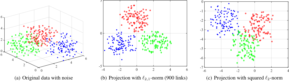
Figure. 1(a) shows three classes, each of which contains 100 data points in ℜ3 . In all, there are 3 × 100 × 99/2 = 14850 point pairs which can be used as must-links and 3 × 100 × 100 = 30000 point pairs which can be used as cannot-links. In our experiments, we randomly select some point pairs to construct three sets consisting of certain number of must-link and cannot-link which correspond to A and B in Eq. (5). We learn the optimized projection matrix W from Algorithm 3. Figure. 1(b)) show the projection in ℜ2 (i.e., y = WT x and W ∈ R3×2 ). We see that the data mixed in the original space from a certain perspective could be separated after projection with certain numbers of links.
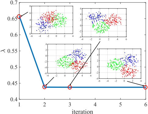
We set the number of links fixed to be 300 and study the projection with update in Algorithm 1. Since we optimize W through an updating method and in each update the objective function monotonically decreases, the clustering of a projection is expected to be better with update. Figure. 2 shows the objective changes through iteration with W initialized randomly. We see that, the objective converges within several iterations, and the clustering becomes better with update which validates our proposed algorithm.
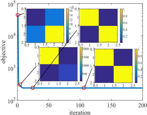
Within each update in Algorithm 1 to optimize W given certain λ, we make use of ADMM to derive W with orthogonal constraint (WT W = I). Figure. 3 demonstrates the objective changes in Eq. (9) through update, we see that our algorithm will get the objective decrease sharply and result in a strictly orthogonal matrix W.
4.2 Application to Real World Data Set Clustering
We first experiment with four benchmark data sets downloaded from the UCI machine learning data repository, including the Breast, Iris, Wine and Ionosphere 2 , and one image data set downloaded from the ORL 3 database, whose details are summarized in Table 2.
2 https://archive.ics.uci.edu/ml/datasets.html
3 http://www.cl.cam.ac.uk/research/dtg/attarchive/facedatabase.html
| Datasets (#data, #classes) | Mah | RCA | DCA | Xiang's | LMNN | ITML | Wang's | KISSME | WDML | Ours |
|---|---|---|---|---|---|---|---|---|---|---|
| MNIST (70000, 10) | 54.69 | 56.12 | 55.04 | 58.76 | 57.61 | 59.87 | 62.04 | 64.76 | 64.61 | 65.87 |
| MIRFlickr (25000, 18) | 30.13 | 32.50 | 33.09 | 33.11 | 32.55 | 34.07 | 35.18 | 38.96 | 39.12 | 39.41 |
| TDT2 (10212, 30) | 18.89 | 19.20 | 19.41 | 19.76 | 20.20 | 21.01 | 22.51 | 27.16 | 26.27 | 26.61 |
| NUS-WIDE (269648, 81) | 10.28 | 10.12 | 11.00 | 11.16 | 11.86 | 12.03 | 13.14 | 14.89 | 14.97 | 15.13 |
| Data set | Breast | Wine | Iris | Iono. | ORL |
|---|---|---|---|---|---|
| # Samples | 569 | 178 | 150 | 351 | 400 |
| Original dimensions | 30 | 13 | 4 | 33 | 10304 |
| # Clusters | 2 | 3 | 3 | 2 | 40 |
| Reduced dimensions | 4 | 6 | 4 | 4 | 80 |
The proposed method has two parameters: the reduced dimensionality of the projected (sub)space r by the transformation of W and the number of (must/cannot) links. We study their impact on the learned distance metrics by performing clustering on the data set from UCI.
For each experimental trial, first we learn the distance metric from the input data by changing the value of r or number of links while fixing the other parameter, then we performKmeans clustering using the learned distance metric. For each different parameter value, we repeat the experiments 20 times to eliminate the difference caused by the initialization of Kmeans clustering. We report the accuracy of the clustering results (Acc) [Xu et al., 2003].
We evaluate the proposed method on noisy data with outlier samples using the four UCI data sets. We compare our method against its two closest counterparts, including (1) the Euclidean distance (EU) that sets M = I and (2) the standard Mahalanobis distance (Mah) that sets the distance metric as the inverse of the sample covariance matrix, i.e. M = (Cov (X))-1 . We also compare our method against several related and more recent metric learning methods, including (3) RCA method [Bar-Hillel et al., 2003], (4) DCA method [Hoi et al., 2006], (5) Xiang's method [Xiang et al., 2008], (6)Information-Theoretic Metric Learning (ITML) method [Davis et al., 2007], (7) Wang's method [Wang et al., 2014b], (8)KISSME [Koestinger et al., 2012], (9) LMNN [Weinberger and Saul, 2009] and (10) WDML [Li and Tang, 2015]. We implement these compared methods following their original papers, and fine tune their parameters to achieve the best clustering accuracy in independent preliminary experiments. Once the distance metric is learned by a method on a data set, K-means clustering is performed on the same data using the learned distance metric.
| OriginalNoisy | Diff. | OriginalNoisy | Diff. | |||
|---|---|---|---|---|---|---|
| Breast data | Ionosphere data | |||||
| Eu | 86.99 | 81.43 | 6.39% | 77.21 | 73.50 | 4.80% |
| Mah | 89.28 | 84.09 | 5.81% | 80.06 | 76.63 | 4.28% |
| RCA | 90.16 | 85.41 | 5.26% | 81.48 | 79.77 | 2.10% |
| DCA | 90.69 | 86.12 | 5.04% | 83.76 | 80.61 | 3.87% |
| Xiang's | 91.04 | 88.93 | 2.32% | 85.19 | 81.75 | 4.04% |
| ITML | 91.26 | 89.24 | 2.21% | 86.21 | 82.67 | 4.11% |
| LMNN | 90.83 | 88.53 | 2.53% | 85.72 | 82.48 | 3.78% |
| KISSME | 90.45 | 88.19 | 2.5% | 85.89 | 83.22 | 3.11% |
| WDML | 90.89 | 88.43 | 2.7% | 86.90 | 83.78 | 3.56% |
| Wang's | 91.71 | 89.95 | 1.92% | 87.94 | 84.48 | 3.93% |
| Ours | 92.27 | 90.74 | 1.66% | 89.46 | 88.32 | 1.27% |
| Iris data | Wine data | |||||
| Eu | 85.52 | 80.41 | 5.97% | 90.07 | 86.74 | 3.70% |
| Mah | 94.42 | 89.44 | 5.27% | 92.70 | 89.16 | 3.82% |
| RCA | 95.91 | 89.40 | 6.79% | 93.26 | 90.71 | 2.73% |
| DCA | 96.54 | 90.15 | 6.62% | 94.38 | 91.90 | 2.63% |
| Xiang's | 96.60 | 91.24 | 5.55% | 95.51 | 92.42 | 3.24% |
| ITML | 96.27 | 92.95 | 3.45% | 95.44 | 92.48 | 3.10% |
| LMNN | 96.33 | 92.88 | 3.58% | 95.61 | 92.39 | 3.37% |
| KISSME | 96.40 | 92.94 | 3.59% | 95.57 | 93.07 | 2.62% |
| WDML | 96.36 | 93.12 | 3.36% | 95.68 | 93.1 | 2.70% |
| Wang's | 96.57 | 93.53 | 3.15% | 95.90 | 93.18 | 2.83% |
| Ours | 96.78 | 95.23 | 1.60% | 96.63 | 95.07 | 1.61% |
We conduct experiments in following two conditions: (1) original data and (2) noisy data with outlier samples. To emulate the outlier data samples, given the input data set X = [x1, . . . , xn] ∈ Rd×n , we corrupt it by a noise matrix ˜X ∈ Rd×n whose element are i.i.d. standard Gaussian variables. Then, we carry out the same learning and clustering procedures on X + σ ˜X as those on the original data, where σ = δ ‖X‖F ‖ ˜X‖F and δ is a given noise factor. In all our experiments, we set δ = 0.1. For every experimental case, the clustering performance is measured by averaging over 20 trials to eliminate the difference in initializing the K-means clustering procedures, which are reported in Table 3.
We have the following interesting observations. First, our method is consistently better than all other compared methods on all four experimental data sets, which demonstrates that our method is able to learn an effective distance metric that can improve clustering performance. Second, although the improvements by our method over the competing methods on the original data are small, the improvement on data with outliers is much larger. This observation clearly demonstrates the robustness of our method against outlier data samples and empirically justifies our motivation to use the ℓ2,1-norm distance to improve distance metric learning.
We also conduct the experiments on large datasets, including MNIST 4 , MIRFlicker 5 , TDT2 6 and NUS-WIDE 7 , and find that our proposed method is again clearly better than its competing counterparts as reported in Table 1.
4.3 Visual Retrieval on ORL Data Set
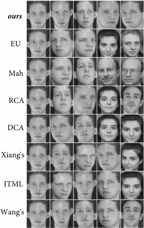
In addition to above comparisons, we also qualitatively evaluate the visual retrieval performance by different metric learning methods. The ORL data set includes 40 distinct individuals and each individual has 10 gray images with different expressions and facial details. The size of each image in this data set is 112×92. When the optimal Mahalanobis distance matrix is learned by side information through links, we calculate the new distance between each image to others and sort them in ascending order and use the first nine ranks to estimate the projection performance. Figure. 4 shows the results of visual comparison for a certain query case. In the figures, the first image in each row is the query image and among the other four, the first two are the closest distance after projection while the last two rank 8-9th closest. From the results, we can see that, our proposed technique returned considerably more relevant images in the top ranked results, which are consistent to the previous quantitative evaluation results.
5 Conclusion
We proposed a robust distance metric learning method using the ℓ2,1-norm distance, which formulated a simultaneous ℓ2,1-norm minimization and maximization (minmax) problem. The new objective uses the ℓ2,1-norm to calculate distance between data points, thus our method is more robust to data outliers. However, the new objective is much more challenging to optimize. To solve this new objective, we derived an efficient algorithm and rigorously proved its convergence. We have performed extensive experiments on both noiseless and noisy data, which have shown our proposed method is superior to traditional methods.
@inproceedings{ijcai2019p417,
  title     = {Learning Robust Distance Metric with Side Information via Ratio Minimization of Orthogonally Constrained L21-Norm Distances},
  author    = {Liu, Kai and Brand, Lodewijk and Wang, Hua and Nie, Feiping},
  booktitle = {Proceedings of the Twenty-Eighth International Joint Conference on
               Artificial Intelligence, {IJCAI-19}},
  publisher = {International Joint Conferences on Artificial Intelligence Organization},
  editor    = {Sarit Kraus},
  pages     = {3008--3014},
  year      = {2019},
  month     = {8},
  note      = {Main track},
  doi       = {10.24963/ijcai.2019/417},
  url       = {https://doi.org/10.24963/ijcai.2019/417},
}
TY - CPAPER TI - Learning Robust Distance Metric with Side Information via Ratio Minimization of Orthogonally Constrained L21-Norm Distances AU - Liu, Kai AU - Brand, Lodewijk AU - Wang, Hua AU - Nie, Feiping T2 - Proceedings of the Twenty-Eighth International Joint Conference on Artificial Intelligence, IJCAI-19 PB - International Joint Conferences on Artificial Intelligence Organization PY - 2019 SP - 3008 EP - 3014 DO - 10.24963/ijcai.2019/417 UR - https://doi.org/10.24963/ijcai.2019/417 ER -Copied
Machine-readable versions of this paper, for tools and AI agents:





