
Recurrent Generative Networks for Multi-Resolution Satellite Data: An Application in Cropland Monitoring
Proceedings of the Twenty-Eighth International Joint Conference on Artificial Intelligence. Main track. Pages 2628-2634.
https://doi.org/10.24963/ijcai.2019/365
Keywords
- Machine Learning: Deep Learning
- Machine Learning Applications: Environmental
- Machine Learning: Classification
- Multidisciplinary Topics and Applications: Computational Sustainability
Abstract
Effective and timely monitoring of croplands is critical for managing food supply. While remote sensing data from earth-observing satellites can be used to monitor croplands over large regions, this task is challenging for small-scale croplands as they cannot be captured precisely using coarse-resolution data. On the other hand, the remote sensing data in higher resolution are collected less frequently and contain missing or disturbed data. Hence, traditional sequential models cannot be directly applied on high-resolution data to extract temporal patterns, which are essential to identify crops. In this work, we propose a generative model to combine multi-scale remote sensing data to detect croplands at high resolution. During the learning process, we leverage the temporal patterns learned from coarse-resolution data to generate missing high-resolution data. Additionally, the proposed model can track classification confidence in real time and potentially lead to an early detection. The evaluation in an intensively cultivated region demonstrates the effectiveness of the proposed method in cropland detection.
- [Audebert et al., 2017] Nicolas Audebert, Bertrand Le Saux, and Sébastien Lefèvre. Joint learning from earth observa- tion and openstreetmap data to get faster better semantic maps. In EARTHVISION 2017 CVPR Workshop, 2017.
- [Che et al., 2016] Zhengping Che, Sanjay Purushotham, Kyunghyun Cho, David Sontag, and Yan Liu. Recurrent neural networks for multivariate time series with missing values. arXiv preprint arXiv:1606.01865, 2016.
- [Chen and Stow, 2003] DongMei Chen and Douglas Stow. Strategies for integrating information from multiple spa- tial resolutions into land-use/land-cover classification rou- tines. PE&RS, 2003.
- [Chung et al., 2015] Junyoung Chung, Kyle Kastner, Lau- rent Dinh, Kratarth Goel, Aaron C Courville, and Yoshua Bengio. A recurrent latent variable model for sequential data. In Advances in neural information processing sys- tems, pages 2980-2988, 2015.
- [Gueguen and Hamid, 2015] Lionel Gueguen and Raffay Hamid. Large-scale damage detection using satellite im- agery. In CVPR, 2015.
- [Guindin-Garcia et al., 2012] Noemi Guindin-Garcia, Ana- toly A Gitelson, Timothy J Arkebauer, John Shanahan, and Albert Weiss. An evaluation of modis 8-and 16-day com- posite products for monitoring maize green leaf area index. Agricultural and Forest Meteorology, 161:15-25, 2012.
- [Habibie et al., 2017] Ikhsanul Habibie, Daniel Holden, Jonathan Schwarz, Joe Yearsley, Taku Komura, Jun Saito, Ikuo Kusajima, Xi Zhao, Myung-Geol Choi, Ruizhen Hu, et al. A recurrent variational autoencoder for human mo- tion synthesis. IEEE CG&A, 2017.
- [Inglada et al., 2016] Jordi Inglada, Arthur Vincent, Marcela Arias, and Claire Marais-Sicre. Improved early crop type identification by joint use of high temporal resolution sar and optical image time series. Remote Sensing, 2016.
- [Jia et al., 2017a] Xiaowei Jia, Ankush Khandelwal, Gu- ruprasad Nayak, James Gerber, Kimberly Carlson, Paul West, and Vipin Kumar. Incremental dual-memory lstm in land cover prediction. In Proceedings of the 23rd ACM SIGKDD International Conference on Knowledge Discov- ery and Data Mining, pages 867-876. ACM, 2017.
- [Jia et al., 2017b] Xiaowei Jia, Ankush Khandelwal, Gu- ruprasad Nayak, James Gerber, Kimberly Carlson, Paul West, and Vipin Kumar. Predict land covers with transition modeling and incremental learning. In SIAM International Conference on Data Mining. SIAM, 2017.
- [Jia et al., 2019a] Xiaowei Jia, Sheng Li, Ankush Khandel- wal, Guruprasad Nayak, Anuj Karpatne, and Vipin Ku- mar. Spatial context-aware networks for mining temporal discriminative period in land cover detection. In SIAM In- ternational Conference on Data mining. SIAM, 2019.
- [Jia et al., 2019b] Xiaowei Jia, Guruprasad Nayak, Ankush Khandelwal, Anuj Karpatne, and Vipin Kumar. Classify- ing heterogeneous sequential data by cyclic domain adap- tation: An application in land cover detection. In SIAM International Conference on Data mining. SIAM, 2019.
- [Jia et al., 2019c] Xiaowei Jia, Jared Willard, Anuj Karpatne, Jordan Read, Jacob Zwart, Michael Stein- bach, and Vipin Kumar. Physics guided rnns for modeling dynamical systems: A case study in simulating lake temperature profiles. In Proceedings of the 2019 SIAM In- ternational Conference on Data Mining, pages 558-566.
- [Kingma and Welling, 2013] Diederik P Kingma and Max Welling. Auto-encoding variational bayes. arXiv preprint arXiv:1312.6114, 2013.
- [Kurtz et al., 2012] Camille Kurtz, Nicolas Passat, Pierre Gancarski, and Anne Puissant. Extraction of complex pat- terns from multiresolution remote sensing images: A hi- erarchical top-down methodology. Pattern Recognition, 45(2):685-706, 2012.
- [Lyu et al., 2016] Haobo Lyu, Hui Lu, and Lichao Mou. Learning a transferable change rule from a recurrent neural network for land cover change detection. Remote Sensing, 2016.
- [Mathieu et al., 2015] Michael Mathieu, Camille Couprie, and Yann LeCun. Deep multi-scale video prediction be- yond mean square error. arXiv preprint:1511.05440, 2015.
- [Myint et al., 2011] Soe W Myint, Patricia Gober, Anthony Brazel, Susanne Grossman-Clarke, and Qihao Weng. Per- pixel vs. object-based classification of urban land cover extraction using high spatial resolution imagery. Remote sensing of environment, 115(5):1145-1161, 2011.
- [Waske and Braun, 2009] Björn Waske and Matthias Braun. Classifier ensembles for land cover mapping using multi- temporal sar imagery. ISPRS Journal of Photogrammetry and Remote Sensing, 64(5):450-457, 2009.
- [Yang et al., 2018] Xi Yang, Yuan Zhang, and Min Chi. Time-aware subgroup matrix decomposition: Imputing missing data using forecasting events. In 2018 IEEE In- ternational Conference on Big Data. IEEE, 2018.
- [Zhang et al., 2017a] Yihang Zhang, Peter M Atkinson, Xi- aodong Li, Feng Ling, Qunming Wang, and Yun Du. Learning-based spatial-temporal superresolution mapping of forest cover with modis images. IEEE Transactions on Geoscience and Remote Sensing, 55(1):600-614, 2017.
- [Zhang et al., 2017b] Yuan Zhang, Chen Lin, Min Chi, Julie Ivy, Muge Capan, and Jeanne M Huddleston. Lstm for septic shock: Adding unreliable labels to reliable predic- tions. In IEEE Big Data. IEEE, 2017.
- [Zhong et al., 2014] Liheng Zhong, Peng Gong, and Gre- gory S Biging. Efficient corn and soybean mapping with temporal extendability: A multi-year experiment using landsat imagery. RSE, 2014.
- [Zhong et al., 2016] Liheng Zhong, Lina Hu, Le Yu, Peng Gong, and Gregory S Biging. Automated mapping of soy- bean and corn using phenology. ISPRS Journal of Pho- togrammetry and Remote Sensing, 2016.
References were extracted automatically from the PDF and may contain errors.
Full text extracted automatically from the PDF; figures, tables and equations may differ. The PDF is the version of record.
1 Introduction
Given the global population growth, an automated cropland monitoring system can offer timely agricultural information which is essential for managing the growing needs of food supply and food security. For example, grain production per acre in United States has doubled from 1975 to 2015 to meet the demand from growing population. These productivity gains are attributable to improved crop varieties and increased planting area. Both of these factors can be captured by an effective monitoring system. Moreover, monitoring croplands has a lot of implications for their environmental sustainability, e.g., the energy consumption for irrigation and the resulting contaminants.
Effective monitoring requires the ability to identify crops over large spatial regions and over long time periods. In recent years, the increasing availability of remote sensing data and advancements in machine learning have created an unrealized potential for analyzing land covers over space and time. Since most land covers have distinct seasonal temporal patterns, sequential models such as Recurrent Neural Networks (RNN) have been widely used to capture these patterns in land cover detection [Jia et al., 2017a; Lyu et al., 2016].
While these sequential models have shown success in leveraging temporal knowledge in classification, they are mostly designed for coarse-resolution remote sensing data, e.g. MODIS (250m, daily). However, the spatial resolution of such data is quite low which makes them unsuitable for monitoring small-scale farms that are quite common in many parts of the world. High-resolution data such as Sentinel (10m, every 10 days in 2016) and Landsat (30m, every 16 days) can be used to monitor small farms, but they are captured less frequently compared to coarse-resolution data. This creates a major issue, especially because remote sensing data is often missing or of poor quality due to clouds and aerosols. For example, Sentinel data are supposed to be available every 10 days (∼ 36 dates in a year), but are available for much less than 25 dates for many locations around the world. If such low quality data is directly used for classification, they are likely to produce bad results. For coarse-resolution data such as from MODIS, a common way to handle this issue is to create composites that aggregate data from multiple dates by selecting the data with the least noise. For example, MODIS 8-day composites are used quite frequently [Guindin-Garcia et al., 2012]. Since high-resolution data are available much less frequently, creating composites such as the ones used for MODIS will result in very infrequent data, making it difficult to capture dynamics of the phenomenon at desired time scale.
In this work, we present a novel framework, Multi-scale Analysis of Remote Sensing data with Missing or poor quality data (MARSM), that combines remote sensing data of different spatial scales, i.e. coarse-resolution and highresolution, to jointly detect/classify croplands. In particular, we utilize MODIS dataset as a coarse-resolution dataset, and Sentinel dataset as a high-resolution dataset. We choose Sentinel over Landsat for its more frequent availability (every 10 days) and better spectrum coverage. We develop a generative sequential model based on variational recurrent neural networks (VRNN) [Chung et al., 2015] on multi-scale data. This model leverages the temporal patterns fromMODIS data to guide the learning process for Sentinel data.
The crop growing process often shows much variability since the crops in different places can have different growing patterns (caused by weather conditions, amount of fertilizer, slope of the land, farmer behaviors). When handling such data with high variability, deterministic sequential models, such as the standard RNN, are known to suffer from the blurry prediction issue [Habibie et al., 2017; Mathieu et al., 2015] by averaging all the possible growing trajectories. In contrast, VRNN ia able to model the variability in crop growing trajectories by introducing latent variables in the internal probabilistic transition structure. For example, consider two corn locations A and B where the corn grows faster in A due to the applied fertilizers. The standard deterministic model will learn a growing pattern of corn to be the average of A and B. In contrast, the VRNN model can automatically sample different latent variables to reflect the difference between A and B and then precisely capture the pattern of each location individually.
Next, we apply the generative process to produce missing Sentinel data. The generation of missing data enables the modeling of a complete crop growing process, which consequently contributes to a better classification. Given the variability in crop growing process, we enforce the generated Sentinel data to conform to true temporal transitions using the guidance of MODIS data and an adversarial regularizer.
Existing detection methods classify land covers only after collecting data from an entire year. However, it is of great interest to governments and companies to obtain the agricultural information at an early stage. We develop a progressive classification method using the outputs from the generative model to track classification confidence in real time. This method can help identify the most discriminative periods for each crop type and thus detect crops at an early stage.
To show the effectiveness in classifying crops and capturing the true growth patterns of each crop type, we evaluate the proposed framework in a crop-intensive region in southwestern Minnesota, US, where high-quality ground-truth is available from USDA Crop Data Layer 1 .
2 ProblemDefinition
In this work, we aim to classify each location at the resolution of a Sentinel pixel (10m×10m) into one of several major crop varieties. The input features include MODIS data (coarseresolution) and Sentinel data (high-resolution), both of which contain multiple time steps in a time period. We fix the time interval to be every 10 days (the same with Sentinel) and utilize MODIS composite images in each 10-day interval. More dataset details will be introduced in Section 4.
For each location, we represent its coarse-resolution MODIS input data as XM={xM1 , xM2 , ..., xMT } with a total of T time steps. For high-resolution Sentinel data, we assume each location has only one missing period between t1 and t2 in method discussion, i.e., XS={xS1 , ..., xSt1 , xSt2 , ..., xST }. However, our proposed method can be easily generalized to handle multiple missing periods in real-world datasets. In our implementation, XM and XS are the data from the MODIS pixel and the Sentinel pixel that cover this location.
Given the multi-scale sequential data collected from certain period, e.g. a year, our objective is to conduct a multiclass classification and output the posterior probability of class label, p(y|XS ,XM ). Besides, we wish to model the progression of this posterior probability p(y|xS≤t , xM≤t ), also referred to as classification confidence, as time t progresses. This enables the identification of crop types with reasonable accuracy before collecting all the data from the entire period.
1 https://nassgeodata.gmu.edu/CropScape/
3 Method
In this section, we propose a framework to combine multiscale sequential data for classifying crops. We first introduce a generative model for learning temporal patterns and handling missing data. Then we will describe a progressive classification method based on the generative model.
3.1 Recurrent Generative Networks
Since MODIS data and Sentinel data are captured using different optical sensors, we model them separately with two recurrent generative networks. However, we will later show the use of the temporal information learned from the MODIS sequence to assist the generative process of Sentinel data.
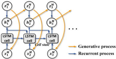
We first build a variational recurrent neural networks (VRNN) on MODIS data (Fig. 1). We will now describe the generative process, recurrent process and inference in details.
The objective of the generative process is to estimate data likelihood p(xM ). We will update model parameters through optimizing the variational lower-bound of log-likelihood. Then given any test data, we can conduct inference of the
latent variables zM , which are then used for classification.
Generative Process
At each time step t, VRNN retains the deterministic hidden representation hMt in standard RNN to store the temporal information. While remote sensing data reflect crop growing process over time, they are also influenced by variability in environmental conditions (including weather as well as nutrients applied by farmers). Therefore, VRNN also introduces latent random variables zM t , which encode the knowledge of underlying crop type and the natural/human factors with influence on spectral features.
The generative process starts with sampling zM t from a Gaussian distribution determined by the information at the previous time step t - 1, as:
where hMt-1 is the hidden representation at t - 1, ϕprior is a trainable function with parameter τ prior (see Section 4.2), diag(·) represents a diagonal variance matrix.
Then we sample xMt , i.e., MODIS data features at t, from a Gaussian distribution with its mean and variance determined by zM t through a function ϕgen , as follows:
Recurrent Process
The hidden representation hMt at time t is obtained through the recurrent procedure, as follows:
where the function Rec(·) is implemented using a LongShort Term Memory (LSTM) with parameter θ in our work, f(xMt ; τ f ) and g(zM t ; τ g ) extract features from rawMODIS data and latent variables (see Section 4.2 for more details). Inference: The direct inference of p(zM t |xMt ) requires the marginalization over zM tractable. Instead, VRNN approximates p(zM Gaussian distribution q(zM mean and variance of q(zM
t , which is computationally int |xMt ) by a t |xMt ) [Chung et al., 2015]. The t |xMt ) are determined by xMt and hMt-1 through a function ϕinf , as follows:
High-resolution Modeling
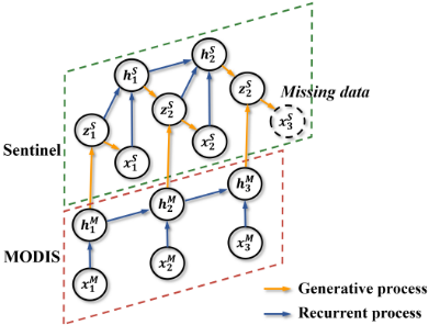
Next, we utilize the temporal information obtained from MODIS data to guide the generative process of Sentinel data. Specifically, the latent variable zS t for Sentinel data depends not only on the high-resolution information by t-1 (encoded by hSt-1 ), but also the temporal patterns of low-resolution data by time t (encoded by hMt ), as shown in Fig. 2. The prior distribution of zS t can be expressed as:
Then we sample xSt from zS t in a similar way with Eq. 2. The generative process involves both the information from previous Sentinel data as well as the MODIS data until current time step. Similarly, the inference process should also involve hMt , which depends on xM≤t . Therefore we have the approximated inference function as q(zS t |xSt , xM≤t ).
Variational Lower-bound
the log-likelihood of multi-scale data can be factorized into two components, corresponding to coarse-resolution data and high-resolution data, respectively.
where the subscript {≤ t1, t2 : T} represents all the available time steps for high-resolution data, i.e., the time steps before t1 and from t2 to T .
Since the marginalization over z is computationally intractable, we alternatively maximize the variational lowerbound of the log-likelihood. By using the fact that q(zM ≤T |xM≤T ) = ∏t q(zM t |xM≤t , zM <t ), and p(xM≤T , zM ≤T ) = ∏t p(xMt |zM ≤t , xM<t )p(zM t |xM<t , zM <t ), we can obtain a variational lower-bound for the coarse-resolution data:
Similarly, we can derive the variational lower-bound for the likelihood of high-resolution Sentinel data log p(xSt=1:t1,t2:T |xM≤T ) as follows:
By approximating the expectation in Eqs. 7 and 8 by the "reparameterization trick" [Kingma and Welling, 2013], the variational lower-bound becomes fully differentiable and can be maximized by the standard back-propagation algorithm.
3.2 Adversarial Data Generation
It is noteworthy that the lower-bound in Eq. 8 only takes the summation over t ≤ t1 and t2 ≤ t ≤ T. However, to compute the distribution at time step t2, we need the information of xSt1+1:t2-1 and hSt1+1:t2-1 . Also, the information in missing period enables the modeling of a complete crop growing process and facilitates the progressive classification described in Section 3.3. Therefore, we generate missing data during the period [t1 +1, t2 -1] in the following way. For each time step t in [t1 + 1, t2 - 1], we first generate zS t by Eq. 5 using hSt-1 and hMt . Then we sample xSt according to the Gaussian distribution determined by zS t (Fig. 2). After obtaining xSt , we compute hSt and the distributions at t + 1.
Due to the potential temporal changes caused by a variety of natural/human factors, a reasonable generative process may output sequential data following t1 in various trajectories with different probabilities. To ensure that the generated data are consistent with the true scenario, we leverage two auxiliary information sources to constrain the data generation. First, as mentioned in Section 3.1, we utilize the coarseresolution data (MODIS) to guide the transition of Sentinel data, as MODIS data is more frequently available. Second, we impose an adversarial regularizer to enforce that the generated data do not deviate from the true data after t2.
Specifically, we repeat the generative process to sample the data after t2. The adversarial regularizer enforces that the generated data and the true data after t2 cannot be easily distinguished by a well trained discriminative classifier D : zS ↦→ [0-true, 1-generated]. Our cost function for the generative model combines the log-likelihood (Eqs. 7 and 8) and the adversarial regularizer with a hyper-parameter λ, as:
where ˆx denotes the generated data. X S t represents the distribution of provided Sentinel data at time t. The selection of hyper-parameters will be discussed in Section 4.2.
3.3 Progressive Classification
After gathering latent variables from the generative model, we utilize them to capture the progression of classification confidence over time. Specifically, we utilize the accumulated discriminative information until time t to make classification decision at t. We expect that the model becomes more and more confident about the classification as time progresses. For location i, the discriminative information at time t is computed from its obtained latent variables [zS i,t , zM i,t ]. Here we add the subscript i to represent the location index. To mitigate the noise at individual locations, we also adopt an isotropic Gaussian smoothing over the spatial neighborhood N(i). In the smoothing process, we use latent variables learned from MODIS data since MODIS data are more robust to noise. More formally, we collect the discriminative information at time t and add it to an accumulated variable oi,t, as:
where γ 2 represents the isotropic variance in the smoothing process, and dm is the dimensionality of zM . W denotes the parameters in sigmoid function to transform latent variables [zS j,t , zM j,t ] to the discriminative information at t.
Then we compute the posterior probability of class label yi by time step t, via a softmax function, as:
The entire framework can be trained using backpropagation algorithm in two stages. In the first stage, we conduct unsupervised training by minimizing the cost function in Eq. 9. Then in the second stage, we fine-tune model parameters in supervised fashion with training labels.
4 Experiment
4.1 Datasets
MODIS. We combine MODISMOD09A1 and MOD09Q1 multi-spectral products, collected by MODIS instruments onboard NASA's satellites. MODIS data are collected for every single day. The dataset provides reflectance values on 7 spectral bands (620-2155 nm) for every location at 250 m resolution. The product MOD09A1 and MOD09Q1 prerprocess the satellite data by filtering precipitable water and cloud. To match the temporal frequency of Sentinel data, we utilize MODIS composite images by selecting per-pixel reflectance values with least noise during each time interval.
Sentinel. Sentinel-2Adata are collected byEuropean Space Agency, which aims to provide global data for every 10 days. The Sentinel-2A data product performs a cloud screening, but does not conduct atmospheric corrections. The data consist of reflectance values on 13 spectral bands, including the visible spectrum, NIR and SWIR. Depending on the spectral bands, the spatial resolution of collected data is 10/20/60 m. In our work, we project all the bands into 10 m spatial resolution. Due to operational or quality issues, many data are missing on certain dates.
Study region. Our study region in southwesternMinnesota covers 490,000 locations at the resolution of Sentinel data, which cover an area of 4,900 ha. We establish the mapping between MODIS and Sentinel and gather the MODIS data for each location. The involved MODIS data in total cover 1,236 MODIS pixels. In the experiment, we only consider major crop types planted in this region, which include corn, soybean and sugarbeet, as their ground-truth labels in USDA crop data layer product are more accurate than other minor crops. Among all the locations in our study region, 217,435 locations are corns, 101,883 locations are soybeans and 96,612 locations are sugarbeets.
4.2 Classification
We first evaluate the classification performance of MARSM. In our implementation, we conduct pixel-wise classification for each location/pixel at Sentinel level (10m×10m). We use two-layer neural networks for functions ϕgen , ϕprior and ϕprior with 120 hidden variables for Sentinel and 80 hidden variables for MODIS. The dimension of the latent variable z is 80 and 60 for Sentinel data and MODIS data, respectively. The hyper-parameter λ in adversarial learning is set to 0.2.
We compare MARSM to multiple baselines, including Artificial Neural Networks (ANN) using concatenated multitemporal data, ensemble single-date Random Forest model (e-RF) [Waske and Braun, 2009], ensemble Fully Convolutional Neural Networks (e-FCNN) [Audebert et al., 2017], and standard LSTM using concatenated multi-scale data at each time step and linear interpolation for missing data.
We also compare against baselines that impute missing data, including GRU-D [Che et al., 2016], and LSTM models using the generated missing data by a temporal-example learning(TEL)-based super-resolution approach [Zhang et al., 2017a] (LSTMtel ) and by the proposed MARSM method (LSTMgen ). Also, we compare against an LSTM combining multi-scale data in the final layer (cLSTM) following [Chen and Stow, 2003] (using generated data by MARSM).
| Entire-region test | Cross-region test | |||||||||||||||
|---|---|---|---|---|---|---|---|---|---|---|---|---|---|---|---|---|
| TA | TA | TB | ||||||||||||||
| Method | Corn | Soy | Sugar | All | Corn | TB Soy | Sugar | All | Corn | Soy | Sugar | All | Corn | Soy | Sugar | All |
| ANN | 0.80 | 0.03 | 0.01 | 0.66 | 0.80 | 0.33 | 0.42 | 0.69 | 0.61 | 0.23 | 0.17 | 0.59 | 0.63 | 0.00 | 0.33 | 0.64 |
| e-RF | 0.77 | 0.57 | 0.82 | 0.75 | 0.81 | 0.78 | 0.84 | 0.81 | 0.73 | 0.60 | 0.53 | 0.66 | 0.72 | 0.63 | 0.63 | 0.69 |
| e-FCNN | 0.80 | 0.59 | 0.82 | 0.78 | 0.81 | 0.83 | 0.83 | 0.82 | 0.70 | 0.61 | 0.58 | 0.66 | 0.74 | 0.63 | 0.62 | 0.72 |
| LSTM | 0.74 | 0.65 | 0.75 | 0.72 | 0.87 | 0.83 | 0.94 | 0.88 | 0.79 | 0.62 | 0.57 | 0.70 | 0.82 | 0.61 | 0.61 | 0.74 |
| LSTMtel | 0.80 | 0.75 | 0.78 | 0.78 | 0.89 | 0.85 | 0.92 | 0.90 | 0.77 | 0.63 | 0.57 | 0.69 | 0.80 | 0.61 | 0.63 | 0.73 |
| LSTMgen | 0.84 | 0.75 | 0.82 | 0.82 | 0.92 | 0.90 | 0.91 | 0.93 | 0.78 | 0.65 | 0.59 | 0.73 | 0.82 | 0.69 | 0.56 | 0.76 |
| cLSTM | 0.88 | 0.80 | 0.79 | 0.85 | 0.91 | 0.88 | 0.94 | 0.92 | 0.77 | 0.62 | 0.66 | 0.73 | 0.83 | 0.62 | 0.58 | 0.76 |
| GRU-D | 0.87 | 0.77 | 0.90 | 0.85 | 0.94 | 0.82 | 0.92 | 0.92 | 0.69 | 0.22 | 0.03 | 0.54 | 0.65 | 0.47 | 0.69 | 0.59 |
| MARSMstn | 0.78 | 0.79 | 0.77 | 0.77 | 0.81 | 0.78 | 0.83 | 0.79 | 0.76 | 0.62 | 0.49 | 0.67 | 0.78 | 0.63 | 0.59 | 0.72 |
| MARSMwadv | 0.90 | 0.82 | 0.82 | 0.87 | 0.89 | 0.90 | 0.84 | 0.90 | 0.80 | 0.61 | 0.60 | 0.74 | 0.82 | 0.63 | 0.61 | 0.75 |
| MARSMwsp | 0.89 | 0.87 | 0.86 | 0.90 | 0.91 | 0.96 | 0.94 | 0.95 | 0.84 | 0.64 | 0.60 | 0.77 | 0.83 | 0.68 | 0.64 | 0.80 |
| MARSM | 0.92 | 0.89 | 0.88 | 0.92 | 0.92 | 0.97 | 0.93 | 0.96 | 0.84 | 0.64 | 0.64 | 0.78 | 0.88 | 0.63 | 0.65 | 0.80 |
We finally compare against three variants of MARSM to show the efficacy of several factors: (1) MOD - incorporation of MODIS data, (2) ADV - adversarial regularizer, and (3) SP - spatial smoothing in classification. These variants are MARSMstn (no MOD, ADV or SP), MARSMwadv (with MOD), MARSMwsp (with MOD+ADV).
We test each method on two periods in 2016: TA - Jan 06 to May 25 with Sentinel data missing on Feb 25, Mar 06, and Mar 16, and TB - Apr 05 to Nov 11 with Sentinel data missing on July 04 and July 14. Note that TA does not cover the crop growing season, but crop residues still show distinctions among different varieties.
For each period, we measure the classification performance by randomly selecting 60% data for training and then testing on the remaining 40% data. Also, we evaluate the performance in two scenarios: 1) entire-region test: the training and testing data are sampled from the same region, i.e., the entire study region, and 2) cross-region test: we randomly select a continuous test region, and then take training samples which do not overlap with test region.
According to Table 1, we observe that the performance in cross-region test is generally worse than that in entire-region test since farmers in different places have different preference in planting and harvesting crops. Besides, the performance in TB is generally better than TA, as TB covers the growing season, which shows more distinctive characteristics of crops.
In both tests, MARSM outperforms the other baselines. The comparison between MARSMstn and MARSMwadv shows that MODIS data can provide promising insights in learning the temporal patterns which contribute to missing data generation and classification. The improvement from MARSMwadv to MARSMwsp shows the effectiveness of the adversarial regularizer. In addition, MARSM outperforms MARSMwsp because it incorporates the spatial smoothing.
Besides, we can observe that ANN does not perform as well as other sequential models. This is because different crops look similar in many single dates. Moreover, the ensemble single-date methods e-RF and e-FCNN do not perform well because they do not make use of the temporal growing patterns. Also, e-RF does not model any interactions between data from two sources.
The comparison between {LSTM, LSTMtel } and {LSTMgen , LSTMcomb } demonstrates that MARSM can generate high-quality data. The direct interpolation used in LSTM baseline or the TEL-based super-resolution approach in LSTMtel suffer from the heavy noise that exists at individual locations in Sentinel data. Also, they can hardly capture the variability of crops. Overall, these methods have lower accuracy than MARSM since the error for generated data can be further accumulated to classification. The method GRU-D imputes missing data based on a decaying factor determined by the data. This method performs well in the entire-region test but cannot generalize to different test regions with shift on the feature space.
4.3 GeneratedMissing Data
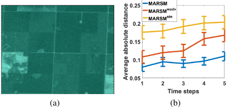
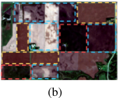
We zoom into a small region and show the generated data on Jul 14 (Fig. 3 (a)). Due to the heavy noise in Sentinel data and the complex relationships among multiple spectral bands, the generated data is slightly blurry compared to true data. Nevertheless, the generated data capture the boundaries of croplands and distinctions between different crops, which are critical to the classification.
To quantify the performance of data generation, we evaluate MARSM, MARSMwadv and MARSMstn by comparing the generated data with true data. Specifically, for each method, we generate data from Jul 24 to Sep 2 (five time steps). Then we measure the average absolute distance between generated data and true data over all the locations. The results are shown in Fig. 3 (b). We observe that the generated data by MARSM stay close to true data over all the five steps. Without adversarial regularizer, MARSMwadv does not perform as well as MARSM, especially after more time steps. On the other hand, as MODIS data provide information of temporal evolution and mitigate the noise in Sentinel data, the removal of MODIS data leads to the generation of less accurate data, as can be seen by the performance of MARSMstn .
4.4 Confidence Progression
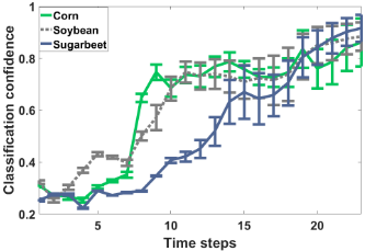
Here we apply MARSM from Apr 05 to Nov 11 (23 time steps). For each class of corn, soybean, and sugarbeet, we measure the classification confidence (averaged over corresponding samples) over time, as shown in Fig. 4.
Our method captures that corn samples quickly gain confidence at the 8th and 9th time steps, which correspond to Jun 14∼Jun 24. To validate the correctness of this finding, we show the RGB image of an example region captured on Jun 24 in Fig. 5 (a). We can clearly see that in the early growing season, corn turns into green more quickly than soybean and sugarbeet, and therefore can be identified in this period.
Fig. 4 shows MARSM detects that sugarbeets still gain confidence after October. We show another RGB image on Oct 05 (the same example region) in Fig. 5 (b). While corns and soybeans have been harvested, sugarbeets still remain green. This demonstrates that MARSM can successfully capture the periods with discriminative knowledge and quickly gains confidence in these periods.
5 RelatedWork
Many existing works map croplands by using MODIS data at 250/500m spatial resolution [Inglada et al., 2016; Zhong et al., 2016], but they cannot identify small crop patches that widely exist in the world. Some other works directly apply machine learning algorithms on high-resolution imagery
(a)
(e.g., Landsat and Sentinel) [Zhong et al., 2014; Inglada et al., 2016], or on the extracted object-based or shape-based features [Gueguen and Hamid, 2015; Myint et al., 2011]. However, these works do not well address the challenges in high-resolution data, including natural noise factors, irregular temporal frequency and low data quality. To solve these challenges, researchers have sought for combining data in different resolutions for detection [Chen and Stow, 2003; Kurtz et al., 2012; Audebert et al., 2017]. However, these works only focus on combining data at single snapshots.
With recent advances of deep learning, RNN-based models have shown to be effective in many land cover and environmental problems [Lyu et al., 2016; Jia et al., 2017a; Jia et al., 2017b; Jia et al., 2019b; Jia et al., 2019a; Jia et al., 2019c]. However, due to their fully deterministic internal transition structure, they are inappropriate to model the variability in data with complex dependencies. To this end, VRNN is proposed which introduces randomness via latent variables and models the dependencies between latent variables at neighboring time steps [Chung et al., 2015]. Our proposed method is based on the VRNN model but extends it to handle multi-scale multi-temporal data and track the realtime confidence progression.
6 Conclusion
In this paper, we propose a framework MARSM that combines multi-scale remote sensing data to identify croplands. The experimental results demonstrate that MARSM greatly improves the detection by learning from multi-scale data. Also, the generated missing data by MARSM stay close to true data over time, and lead to a better classification. In addition, the obtained confidence progression results conform to the growth patterns of crops through visual validation. With the advances in remote sensing technology, the proposed framework can contribute to a large class of land cover problems, which help promote the understanding of global environmental changes.
MARSM can also be applied to other important applications, such as the disease progression modeling where healthcare data are often collected at different time scales with high missing rate [Yang et al., 2018; Zhang et al., 2017b].
Acknowledgements
This work was funded by the NSF awards 1838159 and 1739191. Access to computing facilities was provided by Minnesota Supercomputing Institute.
@inproceedings{ijcai2019p365,
  title     = {Recurrent Generative Networks for Multi-Resolution Satellite Data: An Application in Cropland Monitoring},
  author    = {Jia, Xiaowei and Wang, Mengdie and Khandelwal, Ankush and Karpatne, Anuj and Kumar, Vipin},
  booktitle = {Proceedings of the Twenty-Eighth International Joint Conference on
               Artificial Intelligence, {IJCAI-19}},
  publisher = {International Joint Conferences on Artificial Intelligence Organization},
  editor    = {Sarit Kraus},
  pages     = {2628--2634},
  year      = {2019},
  month     = {8},
  note      = {Main track},
  doi       = {10.24963/ijcai.2019/365},
  url       = {https://doi.org/10.24963/ijcai.2019/365},
}
TY - CPAPER TI - Recurrent Generative Networks for Multi-Resolution Satellite Data: An Application in Cropland Monitoring AU - Jia, Xiaowei AU - Wang, Mengdie AU - Khandelwal, Ankush AU - Karpatne, Anuj AU - Kumar, Vipin T2 - Proceedings of the Twenty-Eighth International Joint Conference on Artificial Intelligence, IJCAI-19 PB - International Joint Conferences on Artificial Intelligence Organization PY - 2019 SP - 2628 EP - 2634 DO - 10.24963/ijcai.2019/365 UR - https://doi.org/10.24963/ijcai.2019/365 ER -Copied
Machine-readable versions of this paper, for tools and AI agents:





