
Multi-view Spectral Clustering Network
Proceedings of the Twenty-Eighth International Joint Conference on Artificial Intelligence. Main track. Pages 2563-2569.
https://doi.org/10.24963/ijcai.2019/356
Keywords
- Machine Learning: Multi-instance;Multi-label;Multi-view learning
- Machine Learning: Clustering
Abstract
Multi-view clustering aims to cluster data from diverse sources or domains, which has drawn considerable attention in recent years. In this paper, we propose a novel multi-view clustering method named multi-view spectral clustering network (MvSCN) which could be the first deep version of multi-view spectral clustering to the best of our knowledge. To deeply cluster multi-view data, MvSCN incorporates the local invariance within every single view and the consistency across different views into a novel objective function, where the local invariance is defined by a deep metric learning network rather than the Euclidean distance adopted by traditional approaches. In addition, we enforce and reformulate an orthogonal constraint as a novel layer stacked on an embedding network for two advantages, i.e. jointly optimizing the neural network and performing matrix decomposition and avoiding trivial solutions. Extensive experiments on four challenging datasets demonstrate the effectiveness of our method compared with 10 state-of-the-art approaches in terms of three evaluation metrics.
- [Andrew et al., 2013] Galen Andrew, Raman Arora, Jeff Bilmes, and Karen Livescu. Deep canonical correlation analysis. In Proc Int Conf Mach Learn, pages 1247-1255, 2013.
- [Cai et al., 2011] Xiao Cai, Feiping Nie, Heng Huang, et al. Heterogeneous image feature integration via multi-modal spectral clustering. In Proc IEEE Conf Comput Vis Pat- tern Recognit, pages 1977-1984. IEEE Computer Society, 2011.
- [Cao et al., 2015] Xiaochun Cao, Changqing Zhang, Huazhu Fu, Si Liu, and Hua Zhang. Diversity-induced multi-view subspace clustering. In Proc IEEE Conf Comput Vis Pat- tern Recognit, pages 586-594, 2015.
- [Deng et al., 2015] Cheng Deng, Zongting Lv, Wei Liu, Jun- zhou Huang, Dacheng Tao, and Xinbo Gao. Multi-view matrix decomposition: A new scheme for exploring dis- criminative information. In Proc Int Joint Conf Artifi In- telli, pages 3438-3444, 2015. IJCAI
- [Elhamifar and Vidal, 2013] Ehsan Elhamifar and Rene Vi- dal. Sparse subspace clustering: Algorithm, theory, and applications. IEEE Trans Pattern Anal Mach Intell, 35(11):2765-2781, September 2013.
- [Hadsell et al., 2006] Raia Hadsell, Sumit Chopra, and Yann LeCun. Dimensionality Reduction by Learning an In- variant Mapping. In Proc IEEE Conf Comput Vis Pat- tern Recognit, pages 1735-1742, New York City, NY, June 2006. IEEE.
- [Hu et al., 2018] Junlin Hu, Jiwen Lu, and Yap-Peng Tan. Sharable and individual multi-view metric learning. IEEE Trans Pattern Anal Mach Intell, 40(9):2281-2288, 2018.
- [Ji et al., 2017] Pan Ji, Tong Zhang, Hongdong Li, Mathieu Salzmann, and Ian Reid. Deep Subspace Clustering Net- works. In Proc Adv Neural Inf Process Syst, Long Beach, US, 2017.
- [Kumar et al., 2011] Abhishek Kumar, Piyush Rai, and Hal Daume. Co-regularized multi-view spectral clustering. In Proc Adv Neural Inf Process Syst, pages 1413-1421, 2011.
- [Li et al., 2015] Yeqing Li, Feiping Nie, Heng Huang, and Junzhou Huang. Large-scale multi-view spectral cluster- ing via bipartite graph. In Proc Conf AAAI Artif Intell, pages 2750-2756, 2015.
- [Liu et al., 2013] Guangcan Liu, Zhouchen Lin, Shuicheng Yan, Ju Sun, Yong Yu, and Yi Ma. Robust recovery of sub- space structures by low-rank representation. IEEE Trans Pattern Anal Mach Intell, 35(1):171-184, 2013.
- [Liu et al., 2015] Xianglong Liu, Lei Huang, Cheng Deng, Jiwen Lu, and Bo Lang. Multi-view complementary hash tables for nearest neighbor search. In Proc IEEE Int Conf Comput Vis, pages 1107-1115, 2015.
- [Lu et al., 2016] Canyi Lu, Shuicheng Yan, and Zhouchen Lin. Convex sparse spectral clustering: Single-view to multi-view. IEEE Trans Image Process, 25(6):2833-2843, 2016.
- [Lu et al., 2018] Canyi Lu, Jiashi Feng, Zhouchen Lin, Tao Mei, and Shuicheng Yan. Subspace clustering by block diagonal representation. IEEE Trans Pattern Anal Mach Intell, 2018.
- [Maaten and Hinton, 2008] Laurens van der Maaten and Ge- offrey Hinton. Visualizing data using t-sne. J Mach Learn Res, 9(Nov):2579-2605, 2008.
- [Ng et al., 2002] Andrew Y Ng, Michael I Jordan, and Yair Weiss. On spectral clustering: Analysis and an algorithm. In Proc Adv Neural Inf Process Syst, pages 849-856, 2002.
- [Nie et al., 2017] Feiping Nie, Jing Li, and Xuelong Li. Self- weighted multiview clustering with multiple graphs. In Proc Int Joint Conf Artifi Intelli, pages 2564-2570, 2017.
- [Peng et al., 2016] Xi Peng, Shijie Xiao, Jiashi Feng, Wei- Yun Yau, and Zhang Yi. Deep subspace clustering with sparsity prior. In Proc Int Joint Conf Artifi Intelli, pages 1925-1931, 2016. IJCAI
- [Peng et al., 2018a] Xi Peng, Jiashi Feng, Shijie Xiao, Wei- Yun Yau, Joey Tianyi Zhou, and Songfan Yang. Structured autoencoders for subspace clustering. IEEE Trans Image Process, 27(10):5076-5086, Oct 2018.
- [Peng et al., 2018b] Xi Peng, Canyi Lu, Yi Zhang, and Hua- jin Tang. Connections between nuclear norm and frobe- nius norm based representation. IEEE Trans Neural Netw. Learn. Syst., 29(1):218-224, Jan. 2018.
- [Shaham et al., 2018] Uri Shaham, Kelly Stanton, Henry Li, Boaz Nadler, Ronen Basri, and Yuval Kluger. Spectral- net: Spectral clustering using deep neural networks. arXiv preprint arXiv:1801.01587, 2018.
- [Vinokourov et al., 2003] Alexei Vinokourov, Nello Cris- tianini, and John Shawe-Taylor. Inferring a semantic rep- resentation of text via cross-language correlation analysis. In Proc Adv Neural Inf Process Syst, pages 1497-1504, 2003.
- [Wang et al., 2015] Weiran Wang, Raman Arora, Karen Livescu, and Jeff Bilmes. On deep multi-view representa- tion learning. In Proc Int Conf Mach Learn, pages 1083- 1092, 2015.
- [Wang et al., 2018] Qi Wang, Mulin Chen, Feiping Nie, and Xuelong Li. Detecting coherent groups in crowd scenes by multiview clustering. IEEE Trans Pattern Anal Mach Intell, 2018.
- [Xu et al., 2013] Chang Xu, Dacheng Tao, and Chao Xu. A survey on multi-view learning. arXiv, April 2013.
- [Yang et al., 2018] Yingzhen Yang, Jiashi Feng, Nebojsa Jo- jic, Jianchao Yang, and Thomas S Huang. Subspace learning by l0-induced sparsity. Proc Int J Comput Vis, 126(10):1138-1156, July 2018.
- [Zhang et al., 2017] Changqing Zhang, Qinghua Hu, Huazhu Fu, Pengfei Zhu, and Xiaochun Cao. Latent multi-view subspace clustering. In Proc IEEE Conf Comput Vis Pattern Recognit, pages 4279-4287, 2017.
- [Zhang et al., 2018] Zheng Zhang, Li Liu, Fumin Shen, Heng Tao Shen, and Ling Shao. Binary multi-view clus- tering. IEEE Trans Pattern Anal Mach Intell, 2018.
- [Zhao et al., 2017] Handong Zhao, Zhengming Ding, and Yun Fu. Multi-view clustering via deep matrix factoriza- tion. In Proc Conf AAAI Artif Intell, pages 2921-2927, 2017.
- [Zhou et al., 2019] Tao Zhou, Mingxia Liu, Kim-Han Thung, and Dinggang Shen. Latent representation learning for alzheimer's disease diagnosis with incomplete multi- modality neuroimaging and genetic data. IEEE Trans Medical Imaging, pages 1-1, 2019.
References were extracted automatically from the PDF and may contain errors.
Full text extracted automatically from the PDF; figures, tables and equations may differ. The PDF is the version of record.
1 Introduction
Clustering is a fundamental task in computer vision and machine learning communities, which aims to cluster data in an unsupervised manner. Over the past decades, a variety of clustering methods have been proposed and recent focus has shifted to handling high-dimensional data that usually lies on a nonlinear low-dimensional manifold. The typical clustering methods include but not limited to spectral clustering or called subspace clustering (SC) [Elhamifar and Vidal, 2013; Liu et al., 2013; Lu et al., 2018; Yang et al., 2018; Peng et al., 2018b] and deep learning based clustering methods [Ji et al., 2017; Peng et al., 2016; Shaham et al., 2018; Peng et al., 2018a]. Although impressive results have been achieved, the aforementioned clustering methods only consider the single-view case while ignoring the information from multiple sources or domains, e.g., image and text. In fact, the object in the real world is usually presented in the form of multi-view and only all views together could represent the object exactly and faithfully. Therefore, it is highly expected to develop multi-view clustering (MvC) approaches to utilize the multi-view information [Hu et al., 2018; Liu et al., 2015; Zhou et al., 2019].
To exploit the diverse and complementary information contained in different views, numerous multi-view clustering methods have been proposed [Xu et al., 2013; Wang et al., 2018], which could be roughly classified into two categories, namely, generative (model-based) methods and discriminative (or similarity-based) approaches. In this paper, we mainly focus on discriminative approaches which learn a set of representations for different views by considering within-view similarity and between-view consistency. The within-view similarity is utilized to learn invariant representation for each single view and the between-view consistency is used to enforce the representations of different views as similar as possible. With the view-specific representation, the clustering results are obtained by conducting some clustering approaches such as k-means on the final representation. In summary, the key to discriminative MvC is formulating the within-view similarity and the between-view consistency.
Based on different formulations of within-view similarity and between-view consistency, discriminative approaches could be further divided into multi-view canonical correlation clustering (MvC3) [Vinokourov et al., 2003], multi-view matrix decomposition clustering (MvMDC) [Deng et al., 2015; Zhao et al., 2017], and multi-view spectral clustering or called multi-view subspace clustering (MvSC) [Kumar et al., 2011; Li et al., 2015; Lu et al., 2016; Wang et al., 2018; Zhang et al., 2017]. Among these methods, MvSC has earned a lot of interests and achieved state-of-the-art performance.
Despite the success of existing MvC works, most of them are nonparametric shallow models which have been proven ineffective and inefficient to handle real-world data, especially considering the large-scale setting and the complex data distribution. To overcome these disadvantages, one promising way is encapsulating deep learning into MvC to utilize the parallel computing fashion and nonlinearity of neural networks. However, only few works have devoted to developing deep multi-view clustering approaches, e.g., deep canonical correlation analysis (DCCA) [Andrew et al., 2013], deep canonically correlated autoencoders (DCCAE) [Wang et al., 2015], and multi-view deep matrix factorization (MvDMF) [Zhao et al., 2017]. On the other hand, although traditional spectral clustering (SC) [Ng et al., 2002] is powerful and widely used, there is no attempt to extend it to the deep neural network framework so far. The main difficulty may lie onto the joint optimization of neural network and the SC loss function. In brief, SC requires solving a matrix decomposition problem, thus making difficulty in jointly optimizing the neural network and the objective function of SC, i.e. the gradient derived from the matrix decomposition cannot be back-propagated to optimize the neural network.
To exploit how to make multi-view spectral clustering benefiting from deep learning, we propose Multi-view Spectral Clustering Network (MvSCN) which aims to learn a common space from multi-view data using a parametric deep model (see Fig. 2). Specifically, MvSCN progressively maps each multi-view data point into a common space with a deep neural network which embraces the local invariance on manifold for each single view and the consistency of pairwise viewspecific representation. The novelty and contribution of this work could be summarized as below:
- Different from traditional SC and MvSC, we propose learning the local invariance by SiameseNet [Hadsell et al., 2006] rather than pairwise local similarity, thus enjoying better clustering performance and smooth cooperation with deep neural network.
- To overcome the aforementioned optimization challenge, we construct an orthogonal layer and propose an optimization method. Note that, the orthogonal layer is generalizable and could be a feasible solution to other matrix decomposition related deep learning, that is be-
- yond the scope of this work and will be investigated in the future.
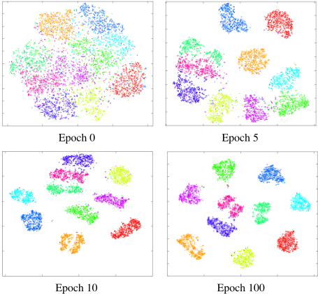
- To the best of our knowledge, the proposed MvSCN could be the first deep extension of multi-view spectral clustering, which is complementary to the classical MvSC. From the view of the classical SC/MvSC, our work may provide a promising way to boost the performance and revive it in the era of big data and deep learning. Fig. 1 presents a visualization result of MvSCN to show its effectiveness and fast convergence.
2 Background and Notations
In this section, we briefly introduce some related works including spectral clustering [Ng et al., 2002] and multi-view spectral clustering [Cai et al., 2011; Kumar et al., 2011]. In this paper, the lower-case mathematical letters denote scalars, the lower-case bold letters denote vectors, the upper-case bold ones denote matrices, and I denotes an identity matrix.
2.1 Spectral Clustering
For a given dataset X = [x1, x2, · · · , xn] ∈ Rd×n , one aims to separate all data points into one of c clusters. Spectral clustering [Ng et al., 2002] first builds an affinity matrix or graph in which each vertex represents a data point, and any two data points are connected i.i.f. one of them is among k nearest neighbors of the other. Specifically, the vanilla spectral clustering method adopts the Euclidean distance with the Gaussian kernel to construct the affinity matrixW as below:
where Wij ∈ W is the connection weight between the i-th and the j-th data point.
With the precomputedW, the objective function of SC is defined by:
where L is a Laplacian matrix defined by L = D - W, D is a diagonal matrix of Dii = ∑j Wij, and Tr(·) denotes the trace of a matrix. The optimal data representation Y to Eq. 2 consists of c eigenvectors corresponding to c smallest eigenvalues of L. With the optimal Y, the clustering assignment is obtained by conducting k-means on it.
2.2 Multi-view Spectral Clustering
Let {X(v) }mv=1 (m ≥ 2) be the v-th view of a dataset. For ease of presentation, considering two-view case, x(1) i and x(2) i denote the same object xi in the first and second views. A general formulation of multi-view based spectral clustering is given in [Li et al., 2015] as below:
where a(v) is the non-negative normalized variable for reflecting the contribution/importance of the v-th view and r is a scalar to control the distribution of different weights on different views. More detail can be seen in [Kumar et al., 2011; Li et al., 2015].
3 Multi-view Spectral Clustering Network
In this section, we propose a deep multi-view clustering method, termed Multi-view Spectral Clustering Network (MvSCN). Different from existing multi-view spectral clustering methods, MvSCN is a deep MvSC which implements the deep neural networks as a parametric function as fθ : Rd → Rc , where d denotes the data dimension, c is the cluster number, and θ denotes the parametric model. Once the representation is obtained with the well-trained θ, k-means is applied to compute the cluster assignments similarly to the traditional MvSC.
3.1 Objective Function
To deeply perform multi-view spectral clustering, we propose the following objective function:
where the within-view similarity L(v) 1 enforces similar points as close as possible in each single view and the between-view consistency L2 aims to learn a common space in which the discrepancy among different views is minimized. λ ∈ [0, 1] is a scalar to balance the contribution of these two losses.
In our objective function, L(v) 1 and L2 encapsulate local invariance on manifold and representation consistency via:
and
where W (v) ij denotes a precomputed similarity graph and y(v) i denotes the output of a neural network w.r.t. the input x(v) i , namely, y(v) i = f (v) θ (x(v) i ), where f (v) θ is the v-th subnetwork θ(v) that is used to handle the v-th view. Note that, we do not explicitly learn a common representation which is close to different view-specific representations. Instead, we learn a common space in which the view-specific representations are as close as possible and obtain the final representation by concatenating the view-specific representations like [Cao et al., 2015; Lu et al., 2016] did. One major advantage of the common space learning is that fewer variables need optimization, thus remarkably decreasing the optimization complexity. In addition, our experimental results will show that such a simple approach could give a favorite clustering result.
In the objective function, L2 (Eq.6) is designed to enforce the view-specific representations of the same data points as similar as possible. L(v) 1 (Eq.5) is designed based on themanifold assumption, i.e., the similarity between the data point x(v) i and its neighbor x(v) j is invariant on manifold in different projection spaces. Clearly, the formulation of W (v) ij plays an important role to the clustering performance. In fact, recent efforts of SC and MvSC have been devoted to this aspect in the context of shallow models, e.g., low rank affinity matrix [Liu et al., 2013; Zhang et al., 2017] and group effect based affinity matrix [Lu et al., 2018]. Different from these methods, we adopt SiameseNet [Hadsell et al., 2006] to learn W (v) ij for improving performance, and will elaborate the implementation in Section 3.2.
Although our network with the above objective function could be easily optimized by the back-propagation algorithm, it will give a trivial solution that maps all inputs to the same point into the common space, i.e.
which makes Eq. 4 achieve the minimizer of 0. In other words, all the data points will collapse into the same point, which is undesirable for clustering task. In order to avoid this issue, a constraint is used to orthogonalize the outputs via
where Y(v) is a n × d matrix in which i-th denotes the y(v) i .
Note that, there are two ways to implement the orthogonal constraint (i.e., Eq. 8). The first one is to incorporate the orthogonal constraint into Eq. 4 as a regularizer, i.e., soft constraint. Such an approach is widely adopted by plenty of shallow models such as SC [Liu et al., 2013; Ng et al., 2002] and MvSC [Kumar et al., 2011; Lu et al., 2016; Zhang et al., 2017], which has suffered from two limitations. On the one hand, a new hyper-parameter is introduced to determine the contribution of the orthogonal term, whose optimal value is hard to find. On the other hand, the soft constraint cannot guarantee the strict orthogonality of Y(v) . Thus, we choose to achieve the orthogonality by recasting the constraint as the top layer of our neural network through the following theorem:
Theorem 1 Given a matrix A and suppose A⊤A is full rank, Q is an orthogonal matrix which is defined as
where L is obtained by Cholesky decomposition as A⊤A = LL⊤ and L is a lower triangular matrix.
Proof For a matrix A that A⊤A is full rank, performing Cholesky decomposition gives A⊤A = LL⊤, where L is a lower triangular matrix. Thus L-1 is lower triangular and (L-1 )⊤ is upper triangular. For Q = A(L-1 )⊤, it is easy to find that Q is an orthogonal matrix by
The proof is complete.
With Theorem 1, we could construct a new layer to implement the orthogonal constraint. To be specific, the orthogonal layer first performs Cholesky decomposition on (Y(v) )⊤Y(v) to obtain L(v) and then obtains the orthogonal The affinity:
W
(v)
Shared Weights
(v)
X
The v-th SiameseNet
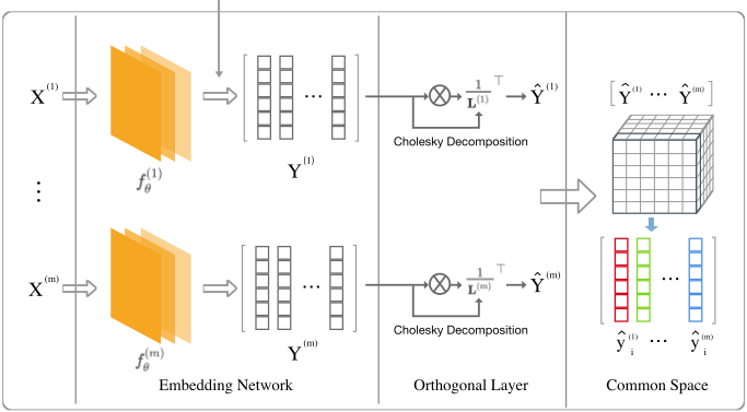
representation via ˆY(v) = Y(v) ((L(v) )-1 )⊤. Note that, the full rankness of (Y(v) )⊤Y(v) could be easily guaranteed by adding a sufficiently small number (e.g., 10-5 ) at the diagonal elements without loss of generality.
3.2 Affinity Learning
Most subspace clustering methods define the local invariance using Euclidean distance with a Gaussian kernel [Ng et al., 2002] or self-expressive representation [Elhamifar and Vidal, 2013; Lu et al., 2016; Yang et al., 2018] from raw data space. Although these methods have shown impressive performance, they may achieve inferior performance when the data distribution is complex. For example, when the data is insufficient sampling.
Different from the aforementioned scheme, we employ SiameseNet [Hadsell et al., 2006] to learn W (v) ij for each view. Given pairs of positive (similar) or negative (dissimilar) samples (xi, xj), SiameseNet learns a parametric model gθ(·) by minimizing the distance of positive pairs while maximizing the distance of negative pairs under the help of the ground-truth. Note that, for ease of representation, we discard the superscript of x(v) i in this section, which will not cause misunderstandings. Formally, the objective function of the SiameseNet is defined as:
where the ground-truth P = 0/1 if the pair (xi, xj) is negative/positive, gθ is a neural network to embed the input xi into a latent space, and γ denotes the distance margin which is fixed to 1.0.
In the unsupervised settings including clustering, however, the ground-truth is unavailable. To solve this issue, we construct the positive and negative pairs using the k-NN graph.
To be exact, (xi, xj) is a positive pair if xj falls into the kneighborhood of xi. To construct the negative pairs, we use xi and its k non-neighbors that are randomly selected. In other words, the positive pairs and the positive pairs are with equal size. Once the SiameseNet achieves convergence, all the data points are passed through the network gθ(·) and the affinity is computed via
3.3 Network Architecture and Training
In this section, we elaborate on the structure and training procedure of our multi-view spectral clustering network. As shown in Fig. 2, the proposed MvSCN consists of two steps involving two networks. The first network learns affinity for each view using a SiameseNet. The second one passes the raw data of each view into an embedding orthogonal space and further projects the view-specific representations into a common space. Note that, these two networks are with only one difference. To be specific, the second one replaces the output layer of the first network with a fully connected layer consisting of c neurons which is followed by the orthogonal layer, where c is the cluster number. More details of the used networks have been presented in the supplementary materials.
We train our network in a coordinate descent fashion which alternates between the orthogonalization and the gradient steps. More specifically,
- Orthogonalization steps: to optimize the orthogonal layer, we use the Cholesky decomposition as shown in Eq. 9 and obtain the orthogonal representations for each view accordingly. Note that, we do not require the orthogonality of cross-batch data points and the Cholesky decomposition cannot guarantee this too. However, the
batch size is usually set to a large number to achieve smooth orthogonalization results.
- Gradient step: for a batch of data, the standard backpropagation is applied to optimize the parameters of the embedding network with the fixed orthogonal layer.
Once our MvSCN achieves convergence, we obtain the final representation by concatenating all view-specific representation together and employ k-means to separate these data into different clusters.
4 Experiment
In this section, we evaluate the performance of the proposed MvSCN. In details, we compare it with 10 state-of-the-art clustering methods including the single view methods: Spectral clustering (SC) [Ng et al., 2002], low rank representation (LRR) [Liu et al., 2013], SpectralNet [Shaham et al., 2018] and the multi-view clustering methods: DCCA [Andrew et al., 2013], DCCAE [Wang et al., 2015], DiMSC [Cao et al., 2015], LMSC [Zhang et al., 2017], MvDMF [Zhao et al., 2017], SwMC [Nie et al., 2017], BMVC [Zhang et al., 2018]. For the single-view clustering methods, we report their results by concatenating the feature vectors corresponding to all views. To further investigate the contributions of components in the proposed model, we define the following three alternative baselines: 1) MvSCN1 : which uses the k-NN graph to compute the affinity matrixW. 2) MvSCN2 : which uses the raw data without data preprocess by the auto-encoder. 3) MvSCN3 : which discards the L2.
All the experiments are implemented using Keras+Tensorflow on a standard Ubuntu-16.04 OS with an NVIDIA 1080Ti GPU. The experiment code will be soon released on Github. In addition, due to space limitation, we provide the full performance comparisons of our method on the supplementary material (https://www.dropbox.com/s/ 48akm1iutn67bdi/SupplementaryMaterial.pdf?dl=0).
4.1 Experiment Setting
We carry out experiments on four popular multi-view datasets including:
- Noisy MNIST 1 : We adopt the setting used in [Wang et al., 2015]. Specifically, we use the original dataset as the view 1, and randomly select within-class images to add additive noisy as the view 2. Thus, we obtain a bi-view dataset consisting of 70K samples for each view.
- Caltech101-20 (A subset of Caltech101 2 ): The dataset consists of 2386 images of 20 subjects. We follow the setting used in [Zhao et al., 2017] to extract six handcrafted features as six views, including Gabor feature, Wavelet Moments, CENTRIST feature, HOG feature, GIST feature and LBP feature.
- Reuters 3 : We use a subset of the Reuters database which consists of the English version and the translations in four different languages, i.e., French, German,
1 http://ttic.uchicago.edu/∼wwang5/dccae.html, createMNIST.m
2 http://www.vision.caltech.edu/Image Datasets/Caltech101/
3 https://archive.ics.uci.edu/ml/datasets.html
Spanish and Italian. The used subset consists of 18758 samples from 6 classes.
- NUS-WIDE-OBJ 4 : This dataset consists of 30K images distributed over 31 classes. We use five features provided by NUS, i.e., Color Histogram, Color Moments, Color Correlation, Edge Distribution and wavelet texture.
For a comprehensive investigation, we adopt Accuracy (ACC), normalized mutual information (NMI), and Fmeasure (F-mea) to evaluate all the tested methods. A higher value indicates a better performance for all metrics.
4.2 Comparisons with State of the Arts
In this section, we compare the proposed MvSCN with 10 state-of-the-art clustering methods on four real-world datasets. To boost the performance and reduce the computational cost, we use a pretrained auto-encoder [Shaham et al., 2018] to reduce the dimensionality for all tested methods. In addition, we use 10K samples randomly selected from Noisy MNIST, Reuters and NUSWIDEOBJ in experiments since most of the baselines are inefficient to handle large-scale dataset. For a fair comparison, we randomly split the dataset into two partitions with equal size, one partition is used to tune parameters for all the methods and the other partition is used for evaluation.
Table 1 shows the quantitative comparison with 10 state-of-the-art methods on four datasets. Note that, as DCCA/DCCAE can only handle bi-view dataset, we report their performance on the best two views accordingly. From Table 1, one could observe that our MvSCN outperforms the compared methods in terms of most the evaluation metrics. Specifically our model achieves 99.18% on Noisy MNIST, which is the best performance to the best of our knowledge. Moreover, our model outperforms compared methods with a large margin on Caltech101-20. Similarly we can see that our method outperforms other methods on Reuters and NUSWIDEOBJ in most cases and LMSC achieves a competitive result in terms of NMI.
4.3 Influence of Parameters
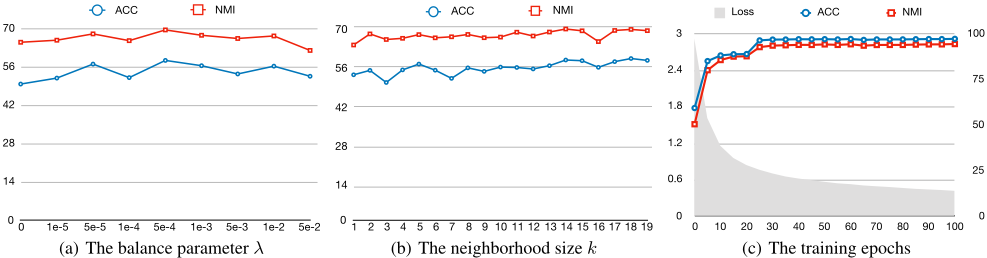
In this section, we investigate the influence of the parameters λ and k of our method. To be specific, MvSCN controls the within-view loss L1 and between-view loss L2 using λ, and uses the neighborhood size k to determine the ground-truth and the connectivity of the affinityW. We conduct the experiment on the Caltech101-20 dataset. As shown in Fig. 3(a), one could see that ACC and NMI firstly increase until about 5 × 10⁻⁵ and then decline with increasing λ. Regarding the parameter k, ACC and NMI of our method almost remain unchanged as shown in Fig. 3(b). In addition, we also investigate the performance w.r.t. training epochs in Fig. 3(c). As shown, the loss consistently decreases with more training epochs, which declines quickly in the first 30 epochs. Regarding ACC and NMI, they first remarkably increase in the first 30 epochs, and then increase smoothly and slowly.
4 http://lms.comp.nus.edu.sg/research/NUS-WIDE.htm
| Noisy MNIST | Caltech101-20 | Reuters | NUSWIDEOBJ | |||||||||
|---|---|---|---|---|---|---|---|---|---|---|---|---|
| Methods | ACC | F-mea | NMI | ACC | F-mea | NMI | ACC | F-mea | NMI | ACC | F-mea | NMI |
| SC | 66.26 | 66.42 | 61.36 | 42.50 | 34.15 | 62.41 | 45.94 | 38.17 | 22.26 | 15.32 | 10.33 | 15.58 |
| LRR | 56.96 | 55.06 | 65.84 | 39.15 | 29.83 | 59.53 | 41.52 | 27.26 | 26.37 | 13.94 | 10.73 | 14.16 |
| SpectralNet | 84.68 | 82.21 | 90.14 | 51.05 | 36.91 | 64.55 | 46.64 | 29.45 | 24.66 | 15.38 | 11.52 | 15.19 |
| DCCA | 95.50 | 95.46 | 89.47 | 42.83 | 37.60 | 62.03 | 29.40 | 25.54 | 6.73 | 16.00 | 8.83 | 11.34 |
| DCCAE | 94.92 | 94.87 | 88.45 | 44.76 | 38.87 | 61.19 | 30.28 | 25.21 | 8.87 | 14.76 | 8.55 | 11.65 |
| DiMSC | 47.24 | 50.25 | 34.84 | 21.46 | 16.59 | 24.70 | 40.50 | 37.38 | 13.51 | 9.28 | 7.49 | 7.53 |
| LMSC | 66.88 | 66.79 | 61.94 | 38.14 | 30.06 | 57.02 | 40.06 | 33.20 | 28.89 | 15.40 | 12.14 | 16.30 |
| MvDMF | 75.26 | 75.00 | 67.12 | 35.96 | 26.23 | 47.25 | 45.78 | 24.93 | 24.69 | 12.04 | 7.49 | 7.53 |
| SwMC | 98.98 | 98.96 | 97.14 | 49.87 | 35.53 | 62.32 | 32.84 | 20.59 | 23.00 | 13.84 | 4.53 | 9.58 |
| BMVC | 90.40 | 85.98 | 93.47 | 36.55 | 25.70 | 56.19 | 46.96 | 34.82 | 22.10 | 14.12 | 9.95 | 12.57 |
| MvSCN1 | 98.12 | 98.08 | 95.63 | 50.38 | 42.01 | 67.10 | 31.02 | 13.58 | 5.46 | 16.08 | 9.67 | 15.24 |
| MvSCN2 | 70.24 | 65.54 | 77.88 | 53.98 | 40.59 | 59.37 | - | - | - | 16.24 | 11.13 | 13.54 |
| MvSCN3 | 84.08 | 81.97 | 89.77 | 45.26 | 36.06 | 63.88 | 47.84 | 40.86 | 25.14 | 13.64 | 9.42 | 14.39 |
| MvSCN | 99.18 | 99.16 | 97.76 | 58.84 | 44.30 | 68.55 | 48.86 | 43.45 | 26.75 | 16.56 | 12.02 | 16.73 |
5 Conclusion
In this paper, we proposed a deep multi-view clustering method, termed as multi-view spectral clustering network (MvSCN) which could be the first deep multi-view spectral clustering. Thanks to the collaboration of the within-view invariance, the between-view consistency, the nonlinear embedding network, and the orthogonal layer, MvSCN could learn a common space in which a discriminative representation is obtained to facilitate the clustering performance. Extensive experiments have shown the efficacy of MvSCN compared to 10 state-of-the-art clustering methods on four challenging datasets. In this work, the orthogonal layer is designed to solve the gradient back-propagation problem and trivial solution caused by cooperation of matrix decomposition and neural network. In the future, we plan to investigate the possibility and solution of implementing the constraints such as low-rankness as a neural model.
Acknowledgments
Corresponding authors are X. Peng and H. Zhu. The work was supported in part by the Fundamental Research Funds for the Central Universities under Grant YJ201949 and 2018SCUH0070, in part by the NFSC under Grant 61806135, 61625204, 61836006, and 61602337, and in part by the grant A1687b0033 and A18A1b0045 from the Singapore government's Research, Innovation and Enterprise 2020 plan (Advanced Manufacturing and Engineering domain).
@inproceedings{ijcai2019p356,
  title     = {Multi-view Spectral Clustering Network},
  author    = {Huang, Zhenyu and Zhou, Joey Tianyi and Peng, Xi and Zhang, Changqing and Zhu, Hongyuan and Lv, Jiancheng},
  booktitle = {Proceedings of the Twenty-Eighth International Joint Conference on
               Artificial Intelligence, {IJCAI-19}},
  publisher = {International Joint Conferences on Artificial Intelligence Organization},
  editor    = {Sarit Kraus},
  pages     = {2563--2569},
  year      = {2019},
  month     = {8},
  note      = {Main track},
  doi       = {10.24963/ijcai.2019/356},
  url       = {https://doi.org/10.24963/ijcai.2019/356},
}
TY - CPAPER TI - Multi-view Spectral Clustering Network AU - Huang, Zhenyu AU - Zhou, Joey Tianyi AU - Peng, Xi AU - Zhang, Changqing AU - Zhu, Hongyuan AU - Lv, Jiancheng T2 - Proceedings of the Twenty-Eighth International Joint Conference on Artificial Intelligence, IJCAI-19 PB - International Joint Conferences on Artificial Intelligence Organization PY - 2019 SP - 2563 EP - 2569 DO - 10.24963/ijcai.2019/356 UR - https://doi.org/10.24963/ijcai.2019/356 ER -Copied
Machine-readable versions of this paper, for tools and AI agents:





