
Monitoring of a Dynamic System Based on Autoencoders
Proceedings of the Twenty-Eighth International Joint Conference on Artificial Intelligence. Main track. Pages 1836-1843.
https://doi.org/10.24963/ijcai.2019/254
Keywords
- Multidisciplinary Topics and Applications: Real-Time Systems
- Machine Learning: Time-series;Data Streams
- Machine Learning Applications: Other Applications
- Knowledge Representation and Reasoning: Diagnosis and Abductive Reasoning
- Machine Learning Applications: Applications of Unsupervised Learning
Abstract
Monitoring industrial infrastructures are undergoing a critical transformation with industry 4.0. Monitoring solutions must follow the system behavior in real time and must adapt to its continuous change. We propose in this paper an autoencoder model-based approach for tracking abnormalities in industrial application. A set of sensors collects data from turbo-compressors and an original two-level machine learning LSTM autoencoder architecture defines a continuous nominal vibration model. Normalized thresholds (ISO 20816) between the model and the system generates a possible abnormal situation to diagnose. Experimental results, including hyper-parameter optimization on large real data and domain expert analysis, show that our proposed solution gives promising results.
- [Alain and Bengio, 2014] Guillaume Alain and Yoshua Ben- gio. What regularized auto-encoders learn from the data- generating distribution. JMLR, 15(1):3563-3593, 2014.
- [Ali et al., 2015] Jaouher Ben Ali, Nader Fnaiech, Lotfi Saidi, Brigitte Chebel-Morello, and Farhat Fnaiech. Ap- plication of empirical mode decomposition and artificial neural network for automatic bearing fault diagnosis based on vibration signals. Applied Acoustics, 89:16-27, 2015.
- [Bach and Maloof, 2008] Stephen H Bach and Marcus A Maloof. Paired learners for concept drift. In Eighth IEEE International Conference on Data Mining, 2008., pages 23-32. IEEE, 2008.
- [Bengio et al., 2015] Samy Bengio, Oriol Vinyals, Navdeep Jaitly, and Noam Shazeer. Scheduled sampling for se- quence prediction with recurrent neural networks. In NIPS, pages 1171-1179, 2015.
- [Borghesi et al., 2018] Andrea Borghesi, Andrea Bar- tolini, Michele Lombardi, Michela Milano, and Luca Benini. Anomaly detection using autoencoders in high performance computing systems. arXiv preprint arXiv:1811.05269, 2018.
- [Cooijmans et al., 2016] Tim Cooijmans, Nicolas Bal- las, César Laurent, C ¸aglar Gülc ¸ehre, and Aaron Courville. Recurrent batch normalization. arXiv preprint arXiv:1603.09025, 2016.
- [Djaidir et al., 2017] Benrabeh Djaidir, Ahmed Hafaifa, and Abdallah Kouzou. Faults detection in gas turbine rotor us- ing vibration analysis under varying conditions. Journal of Theoretical and Applied Mechanics, 55(2):393-406, 2017.
- [Elsken et al., 2018] Thomas Elsken, Jan Hendrik Metzen, and Frank Hutter. Neural architecture search: A survey. arXiv preprint arXiv:1808.05377, 2018.
- [Gal and Ghahramani, 2016] Yarin Gal and Zoubin Ghahra- mani. A theoretically grounded application of dropout in recurrent neural networks. In NIPS, pages 1019-1027, 2016.
- [Greff et al., 2017] Klaus Greff, Rupesh K Srivastava, Jan Koutník, Bas R Steunebrink, and Jürgen Schmidhuber. Lstm: A search space odyssey. IEEE transactions on neural networks and learning systems, 28(10):2222-2232, 2017.
- [Head et al., 2018] Tim Head, MechCoder, Gilles Louppe, Iaroslav Shcherbatyi, et al. scikit-optimize/scikit- optimize: v0.5.2, March 2018.
- [Hinton and Salakhutdinov, 2006] Geoffrey E Hinton and Ruslan R Salakhutdinov. Reducing the dimensionality of data with neural networks. science, 313(5786):504-507, 2006.
- [Hochreiter and Schmidhuber, 1997] Sepp Hochreiter and Jürgen Schmidhuber. Long short-term memory. Neural computation, 9(8):1735-1780, 1997.
- [Hoos and Leyton-Brown, 2014] Holger Hoos and Kevin Leyton-Brown. An efficient approach for assessing hy- perparameter importance. In International Conference on Machine Learning, pages 754-762, 2014.
- [Ioffe and Szegedy, 2015] Sergey Ioffe and Christian Szegedy. Batch normalization: Accelerating deep network training by reducing internal covariate shift. In International Conference on Machine Learning, volume 37, pages 448-456.
- PMLR, 2015.
- [Isermann, 2005] Rolf Isermann. Model-based fault- detection and diagnosis-status and applications. Annual Reviews in control, 29(1):71-85, 2005.
- [Kingma and Ba, 2014] Diederik P Kingma and Jimmy Ba. Adam: A method for stochastic optimization. arXiv preprint arXiv:1412.6980, 2014.
- [Lee et al., 2015] Jay Lee, Behrad Bagheri, and Hung-An Kao. A cyber-physical systems architecture for industry 4.0-based manufacturing systems. Manufacturing Letters, 3:18-23, 2015.
- [Lees et al., 2009] AW Lees, JK Sinha, and MI Friswell. Model-based identification of rotating machines. Mechan- ical Systems and Signal Processing, 23(6):1884-1893, 2009.
- [Li et al., 2000] Bo Li, M-Y Chow, Yodyium Tipsuwan, and James C Hung. Neural-network-based motor rolling bear- ing fault diagnosis. IEEE transactions on industrial elec- tronics, 47(5):1060-1069, 2000.
- [Lin et al., 2017] Tao Lin, Tian Guo, and Karl Aberer. Hy- brid neural networks for learning the trend in time series. In Proceedings of the Twenty-Sixth International Joint Conference on Artificial Intelligence, IJCAI-17, pages 2273-2279, 2017. IJCAI
- [Maaten and Hinton, 2008] Laurens van der Maaten and Ge- offrey Hinton. Visualizing data using t-sne. JMLR, 9(Nov):2579-2605, 2008.
- [Ng, 2011] Andrew Ng. Sparse autoencoder. CS294A Lec- ture notes, 72(2011):1-19, 2011.
- [Osmani and Hamidi, 2018] Aomar Osmani and Massinissa Hamidi. Hybrid and convolutional neural networks for lo- comotion recognition. In Proceedings of the 2018 ACM UbiComp/ISWC 2018 Adjunct, pages 1531-1540. ACM, 2018.
- [Osmani et al., 2017] Aomar Osmani, Massinissa Hamidi, and Abdelghani Chibani. Machine learning approach for infant cry interpretation. In (ICTAI), 2017 IEEE 29th In- ternational Conference on, pages 182-186. IEEE, 2017.
- [Paszke et al., 2017] Adam Paszke, Sam Gross, Soumith Chintala, Gregory Chanan, Edward Yang, Zachary De- Vito, Zeming Lin, Alban Desmaison, Luca Antiga, and Adam Lerer. Automatic differentiation in pytorch. 2017.
- [Qi et al., 2017] Yumei Qi, Changqing Shen, Dong Wang, Juanjuan Shi, Xingxing Jiang, and Zhongkui Zhu. Stacked sparse autoencoder-based deep network for fault diagno- sis of rotating machinery. IEEE Access, 5:15066-15079, 2017.
- [Rahmoune et al., 2017] Mohamed Ben Rahmoune, Ahmed Hafaifa, and Mouloud Guemana. Fault diagnosis in gas turbine based on neural networks: Vibrations speed ap- plication. In Advances in Acoustics and Vibration, pages 1-11. Springer, 2017.
- [Rifai et al., 2011] Salah Rifai, Pascal Vincent, Xavier Muller, Xavier Glorot, and Yoshua Bengio. Contractive auto-encoders: Explicit invariance during feature extrac- tion. In Proceedings of the 28th International Conference on Machine Learning, pages 833-840. Omnipress, 2011.
- [Santurkar et al., 2018] Shibani Santurkar, Dimitris Tsipras, Andrew Ilyas, and Aleksander Madry. How does batch normalization help optimization?(no, it is not about in- ternal covariate shift). arXiv preprint arXiv:1805.11604, 2018.
- [Snoek et al., 2012] Jasper Snoek, Hugo Larochelle, and Ryan P Adams. Practical bayesian optimization of ma- chine learning algorithms. In NIPS, pages 2951-2959, 2012.
- [Tidriri et al., 2016] Khaoula Tidriri, Nizar Chatti, Sylvain Verron, and Téodor Tiplica. Bridging data-driven and model-based approaches for process fault diagnosis and health monitoring: A review of researches and future chal- lenges. Annual Reviews in Control, 42:63-81, 2016.
- [Tobon-Mejia et al., 2012] Diego Alejandro Tobon-Mejia, Kamal Medjaher, Noureddine Zerhouni, and Gerard Tripot. A data-driven failure prognostics method based on mixture of gaussians hidden markov models. IEEE Trans- actions on reliability, 61(2):491-503, 2012.
References were extracted automatically from the PDF and may contain errors.
Full text extracted automatically from the PDF; figures, tables and equations may differ. The PDF is the version of record.
1 Introduction
Condition monitoring of large industrial equipment is critical and becomes more complex because of the integration of new technological artifacts as part of the industry 4.0 transformations [Lee et al., 2015]. Different approaches are used for monitoring these kinds of industrial equipment and can be categorized into model-based, data-driven, and experiencebased approaches [Tobon-Mejia et al., 2012]: (1) Modelbased approaches rely on analytical and physical models in order to represent the behavior of the system [Lees et al., 2009], (2) Data-driven approaches exploit signal processingbased techniques in order to extract discriminative features from sensor signals which, then, are used to build statistical models [Tobon-Mejia et al., 2012] and (3) Experience-based, for their part, are used when no physical model nor sufficient data is available. Typically, these approaches make use of failure history (data loggers) of the industrial equipment on which statistical distribution is fitted in order to establish maintenance schedules.
The applicability of these approaches is usually assessed based on three criteria including cost, precision, and complexity. Data-driven approaches are suitable for large-scale and complex systems. However, performances of the behavior models degrade as the underlying data distribution (used during training phase) shifts from its original form through time. Model-based approaches require an explicit mathematical model. These approaches are more precise than datadriven ones as far as an accurate mathematical model is available which tends to become more difficult and costly given the fact that industrial systems become more complex [Tidriri et al., 2016].
∗Contact Author
Vibration control of rotating machinery is a complex domain especially for large equipment and their continuous control is considered highly strategic. Two main methods exist to monitor these kinds of machines: The first one is a selective approach based on the periodic monitoring of the vibration levels by the use of data loggers. The processing of these data is done offline. Signals are measured between two control periods and any anomaly is obtained by a drift spectrum analysis. The control is carried out point by point according to a previously defined topography. The mathematical tools used are limited to the signal processing applied to the collected signal. The second method is a continuous control of the so-called strategic equipment. In fact, the point collectors of the data are replaced by complex monitoring systems associated with mathematical models for diagnosis.
Several works deal with the condition monitoring problem in particular on rotating machinery [Rahmoune et al., 2017; Ali et al., 2015; Qi et al., 2017]. Some of these works use neural network models as [Li et al., 2000], where the problem is to detect motor rolling bearing faults by using a set of frequency-domain features. More recently, [Ali et al., 2015] exploit capabilities of neural networks and a set of time-frequency domain features in order to characterize and classify various bearing classes. [Rahmoune et al., 2017] for their part generate residues from a gas turbine vibration signals which are then classified using a neural network model. In recent years, the expansion of deep learning approaches has also reached this area. As the success on various real applications of hybrid neural network architectures to learn trends in time series proposed in [Lin et al., 2017; Osmani and Hamidi, 2018; Osmani et al., 2017] and to detect anomalies in high-performance computing systems [Borghesi et al., 2018]. More specifically, the autoencoder solution for fault-diagnosis of rotating machinery proposed in [Qi et al., 2017] where rather than encoding the raw sensor signals, authors in this work apply ensemble empirical mode decomposition and compute autoregressive parameters that are then fed into an autoencoder to learn interesting structures about the input signals.
Figure 1 shows our real application of monitoring of an industrial turbo-compressor system. We notice that there are four major causes for rotor vibrations in gas turbines [Djaidir et al., 2017]: unbalance of the rotor, rapid braking of the shaft, mechanical failure (such as a broken blade), and permanent deformation of the rotor. These vibrations, in turn, cause bearings' rapid deterioration. The analysis of magnitude and harmonics spectrum of signals resulting from measured vibrations are fundamental to detect turbines failures. The objective is to continuously monitor the turbo-compressor torque movement where an optimum operating period is usually selected by experts to take the reference values expressed by a noise level.
In this work, we are interested in developing a monitoring model based on data analysis and machine learning approach to monitor continuously system vibration and to take into account normal evolution in the system by adding a continuous learning level able to follow the evolution of the monitored system. Our original two-level architecture is organized as follow: an autoencoder model [Hinton and Salakhutdinov, 2006] based on long short-term memory units (LSTM) [Hochreiter and Schmidhuber, 1997] tracks in a continuous fashion a set of vibration signals generated by sensors associated to the turbo-compressor operating in real industrial conditions. the second level regularly produces a new generation of autoencoders integrating more data and better adapted to the evolution of the system. It uses the current autoencoder and new non-faulty monitored data to improve the quality of the current autoencoder.
One of the basic limitations of model-based diagnostics is to get a nominal model which faithfully reproduces the behavior of the system. We propose in this paper, a nominal vibration model of the turbo-compressor application by using an autoencoder enabled with automatic cropping capabilities. Experimental results show that this promising approach allows automatic modeling of the system by adapting to changes without the usual efforts required to build a model.
This paper is organized as follow: Section 2 describes the main architecture of the operational application concerned with this study. Section 3 gives details about our approach including using LSTM models, continuous learning and hyperparameters optimization. The encouraging obtained results are summarized in Section 4. Section 5 concludes the paper and gives some perspectives.
2 Application Description
The considered monitoring system is composed of a set of sensors placed around the turbo-compressor according to a manufacturer predefined topology (see Figure 1). The complete system is connected to a real time Bentley Nevada data acquisition platform. The turbine is linked to the compressor via a rigid coupling. In fact, the turbine ensures the rotational drive of the compressor to convey a process gas. The installed sensors essentially measure axial and radial displacements for stability monitoring. It is important to notice that there could be operating conditions in the overall turbocompressor torque integration process affecting the stability of the installation. Continuous control is needed. The control of the stability of the system is ensured by 11 sensors measuring the dynamics of the movement. The measurement of each of sensor must remain inside the boundaries defined by the standard ISO 20816 which defines the maximum threshold expressed in (mm/S RMS). Within the defined limits, each sensor delivers a vibration level independent from others, it depends on the direction of movement of the system and also the noise level of the sensor. Measurement associated with the various sensors have been separately identified for the turbine and for the compressor.
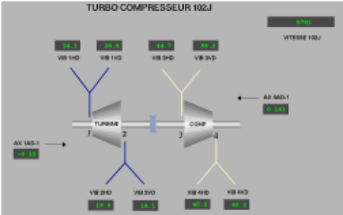
Turbine sensors are: the axial displacement measurement of the turbine (AX 1AD-1), the upper level axial horizontal displacement measurement of the turbine (VIB 1HD), the upper level vertical axial displacement measurement of the turbine (VIB 1BD), the lower level axial horizontal displacement measurement of the turbine (VIB 2HD), the lower level axial horizontal displacement measurement of the turbine (VIB 2HD) and the lower level turbine vertical axial displacement measurement (VIB 2VD). The compressor sensors are: the axial displacement measurement of the compressor (AX 4AD-1), the upper level compressor horizontal axial displacement measurement (VIB 3HD), the upper level vertical axial displacement measurement of the compressor (VIB 3VD), the lower level horizontal axial displacement measurement of the compressor (VIB 4HD), and the lower level vertical axial displacement measurement of the compressor. We use also a common measurement of the rotation speed of the turbine-compressor (102J).
The measurements delivered by the acquisition system are expressed in mm, the thresholds in mm/S RMS and the sampling period is 1s. According to the ISO 20816 standard, the turbo-compressor system belongs to group 4: so the limits (v0) are (1) Not allowed red limit (up to 18mm/S RMS), (2) Threshold Limit defined between 7.1 and 18mm/S RMS, (3) Average Threshold are between 2.8 and 7mm/S RMS and finally (4) Good threshold for vibrations less than 2.8mm/S RMS.
3 Proposed Approach
We are interested in predicting abnormal vibratory phenomena in gas turbines that are susceptible to accelerate the deterioration of the system's components. Specifically, we model the vibration phenomena using a neural network-based autoencoder which is presented first along with the continuous monitoring solution that we provide. This is followed then, by the Bayesian optimization of the hyper-parameters used to tune various parts of the proposed approach.
3.1 Setting
The set of M sensors (also called data generators), denoted {m1, . . . ,mM}, are used to capture the behavior of turbocompressor. Each sensor mi generates a sequence xi = (xi1 , xi2 , . . . ) of vibration observations. Each data generator mi i∈{1..M} is modelled using an LSTM-based autoencoder AEi that is trained via batch gradient descent to minimize a reconstruction error term between an original signal and its reconstruction [Hinton and Salakhutdinov, 2006].
AEs are a non-linear generalization of the principal component analysis. They both belong to the unsupervised representation learning category which "try to characterize the data-generating distribution through the discovery of a set of features or latent variables whose variations capture most of the structure of the data-generating distribution" [Alain and Bengio, 2014]. These latent variables represent what is called the "information bottleneck" in reference to its reduced size which literally forces the model to learn key features from the original signal. This is done through two steps: encoding and decoding which are both based on LSTM unit.
LSTM units are a powerful type of recurrent neural networks that circumvent the long-term dependency problem when it comes to memorizing pieces of information through long periods [Greff et al., 2017]. The main component of these units is the cell state that is designed to the matter of retaining information through long periods of time. Information are added to and removed from this cell state at each time-step t using different gates: the forget gate ft determines the extent to which information is retained from the previous time-step, the input gate it controls the flow of information from the current input xt, and the output gate ot allows the model to read from the cell.
More formally, given an input sequence x = (xt1 , . . . , xt2 ) between two predefined time periods t1 and t2, regardless of the data generator, at each time-step, the current cell state ct, as well as the current hidden state ht are computed using the previous cell state ct-1 and the current input sample, as:
where the matrices W represent the weights of the network and b the biases. The subscripts correspond to their respective gate; for example Whi is the hidden-input gate matrix, Wio is the input-output gate matrix, etc. These are learned through gradient descent while σ and tanh are the sigmoid and the hyperbolic tangent functions respectively and are used to introduce non-linearities into the model.
3.2 Encoder
The first component encodes an input sequence or a batch of sequences using LSTM units and updates its hidden state according to equations 1. We denote this operation ht = LSTM(ht-1, xt). The last hidden state encapsulates sufficient information about the structure of the whole input sequence that is being processed, to subsequently recover the original sequence via decoding. Each generator is processed separately and yield an encoding cmi at the last time-step t2 using the before last hidden state ht2-1:
In order to diagnose the behavior of the generator mi by adding a set of correlated ones {mj|j ∈ J}J⊆{1,..,M}, an encoding cmJ is learned using the remaining concatenated signals and the hidden state is thus updated as follows
These encodings are also called context vectors especially in the field of machine translation as they capture in some way the meaning or context of a given sequence of words.
3.3 Decoder
The reconstruction of the original signal is monitored by these encodings which represent their condensed representation. For a given sequence, at each time-step, the decoder takes as inputs the encoding cmi (or cmJ ) and either the groundtruth sample or the previously reconstructed sample, which is usually designated as teacher-forcing mode in contrast to the free-running mode [Bengio et al., 2015]. Similarly to the encoder, the hidden state ht is updated:
Let us consider yi = (yi t1 , . . . , yi t2 ) to be the autoencoder's output corresponding to the input sequence xi = (xit1 , . . . , xit2 ) of the data generator mi obtained via a linear projection of the hidden state, we define the overall cost function J with respect to xi and its reconstruction yi to be the mean square error
Forward and backward propagation of the reconstruction error between encoder and decoder components allow the model to minimize the discrepancy between the original signal and its reconstruction and besides that, ends-up with a latent space (the encoding) that captures key features of the data distribution.
3.4 Regularization
The way for the autoencoder to learn generalizable encoding and decoding is to ensure that the number of hidden units is sufficiently restricted. Variants of the original AE models that make use of sparsity, denoising, or contraction were proposed [Rifai et al., 2011] and are a way to free them from the information bottleneck and use encodings that are not necessarily smaller than the input dimensions. We need our autoencoder to be sensitive enough to recreate the original observation but insensitive enough to the training data such that the model learns a generalizable encoding and decoding. In order to explore various latent space representations that are more suitable to our particular context, we impose regularization via the sparsity constraint [Ng, 2011]. It imposes that the activation level of the hidden units remains lowmost of the time. For this, the average activation level ˆ ρj of a given hidden unit j is computed over all training sequences. The goal is to enforce ˆ ρj to be as close as possible to a target sparsity probability ρ (the sparsity parameter which is defined to be close to 0). This is done via the minimization of the Kullback-Leibler (KL) divergence between these two probability distributions
where nhu is the number of hidden units in the LSTM layers. To achieve this, we will add an extra penalty term to our optimization objective controlled by a parameter λ, which imposes the sparsity constraint. The whole model is then trained to minimize both the discrepancy between the original signal and its reconstruction and the divergence between ρ and ˆ ρj :
3.5 Monitoring Process
A fault is defined as an unpermitted deviation of at least one characteristic property of a variable from an acceptable behavior [Isermann, 2005]. Previous steps generate a model of the system from data. During this current process, we control average limits between generated signal from the model and the real system using the θ ISO 20816 fixed parameter presented before, i.e. at each step t, we ensure that:
Where xi(t) (resp. yi(t)) is a signal generated by the sensor mi of the real monitored system (resp. our model) at step t and ϵ(t) is an additional error marge.
To reduce the impact of abrupt change between the system and model outputs without connection to the breakdown situations, the regulation function ϵ(t) is computed as follow: ϵ(t) = α|xi(t) + xi(t - 2) - 2xi(t - 1)|.
Additionally, in practice, industrial systems are under continuous physical degradation and adaptation caused by various environmental as well as operational effects. The learned model evolves over time. We propose the following continuous learning model to follow the normal system evolution.
Algorithm 1 Continuous learning model Inputs: xi(t)i∈{1..M}, ζ, η xi(t): signals generated by sensor mi i∈{1..M} ζ: size of the nominal training period η: size of the nominal control period 1: LetMl be the learning model 2: LetMc be the controller model 3: Let Sv be the set of validated examples 4: Sn ← segmentation(xi(t), ζ) {Sn accumulates generated windows} 5: Ml.fit(Sn) {encode with either Eq. 2 or 3} 6: Mc ← copy(Ml) 7: for t ← ζ +1 to T do 8: yi(t) ←Mc.predict(xi(t)) {multi-step-ahead prediction} 9: if |xi(t) - yi(t)| < θ + ϵ(t) then 10: Sv ∪ {xi(t)} 11: else 12: trigger an alarm 13: increase #discrepancies 14: end if 15: if η samples visited or max. #discrepancies reached then 16: Ml.fit(Sv) 17: Mc ← copy(Ml) 18: Sv ← ∅ 19: end if 20: end for3.6 Continuous LearningModel
The physical system evolves and adapts to the environment (turbocharger support that settles, normal wear of seals, etc.). To solve this problem (summarized in Algorithm 1), we propose a two-level model: the current learned model Mc trained initially on a nominal period is used to monitor the real system, and at the same time all data (signals) validated by this model are considered as training examples for the next generation of the controller model Ml. algorithm inputs are the signals xi(t) i∈{1..M}, the size of the initial nominal training period ζ, and the size of the nominal control period η. Ml learns the nominal behavior of the system via the LSTMbased autoencoder architecture proposed above and starts to make multi-step-ahead predictions based on the incoming sequences. At each time-step, these predictions are compared to the real outputs of the system. Whenever the discrepancy between Mc's predicted output and the real system at timestep t is within the desired region of acceptable behavior, Ml is updated with the value of the current discrepancy.
Predicted outputs lying outside of the region of acceptable behavior are discarded and thus do not participate in updating Ml. In our experiments, we evaluated two strategies to learn the next monitoring model: the one based on a prefixed period of time η and the other based on the evolution of the parameter |xi(t) - yi(t)|. Indeed, the underlying hypothesis is updated only when necessary. This contrasts with approaches that make use for example of alternating learners, a stable learner that learns stable concepts and a reactive one that learns transient concepts from recent windows, in order to implement an explicit forgetting mechanism, e.g. [Bach and Maloof, 2008].
At each step of our proposed approach, setting the right hyper-parameters is a critical aspect. Recent advances in neural architecture search demonstrated noticeable successes in many fields leading in certain cases to state-of-the-art architectures using Bayesian optimization in particular [Elsken et al., 2018]. We tune hyper-parameters via a Bayesian optimization procedure based on Gaussian process as a surrogate model in which the generalization performance of a given learning algorithm is modeled as a sample from a Gaussian process [Snoek et al., 2012].
3.7 Bayesian Optimization of the Hyperparameters
The recognition performance of a given configuration is considered as a function f (x) on some bounded set X (the hyperparameters search space), where x is an instantiation of each hyper-parameter of the neural architecture. In other words, the Bayesian optimization procedure constructs a probabilistic model for the function f(x), for which we seek the minimum, and based on that model, samples the next point of the hyper-parameters search space. Sampling from this model can be done more quickly than from the original function.
Expected improvement EI(x) = -E[f(x) - f(x + t)] is used as an acquisition function in order to direct sampling, at time step t, of areas of the hyper-parameter space where an improvement of the performances is likely to happen. The Gaussian process from which hyper-parameter instances are sampled is updated at each time step with the recognition performance achieved by the induced neural architecture in the considered turbo-compressor monitoring problem.
The size of the hidden states of both the encoder and decoder are optimized. Table 2 summarizes the hyperparameters that are assessed through the Bayesian optimization procedure in the considered application.
4 Experiments
In this section, we evaluate our approach on a real industrial application dataset and demonstrate how it can reliably detect abnormal behavior of such industrial equipment. Hyperparameters of both the reconstruction model and continuous learning algorithm are tuned through a Bayesian optimization procedure using the scikit-optimize library [Head et al., 2018]. Code to reproduce experiments is publicly available 1 . All of our experiments were implemented using pyTorch framework [Paszke et al., 2017] and the following describes the details of experiments and results.
Dataset description. Data were collected from a set of 10 sensors that continuously monitor a 102J turbo-compressor operating in a real application. Figure 1 shows a schematic representation of the sensors deployment topology on the industrial setting. It exhibits, in particular, the location of the 8, vertical and horizontal, vibration sensors as well as the 2 axial displacement sensors relative to the different components of the equipment which allow us to assess defects that can appear in any of the three Cartesian directions. Acquisition of vibration data was carried for each sensor at a sampling rate of 1 Hz which is sensitive enough for capturing vibration trends that may indicate defects. For frame-by-frame analysis, signals are segmented into short-term overlapping windows of various lengths w and overlapping is controlled with a hyper-parameter, the step-size, referred to as s.
1 https://www.github.com/hamidimassinissa/vibration-sae
Training procedure. The weights of the reconstruction model are updated via stochastic gradient descent on minibatches of size bs and we use Adam algorithm [Kingma and Ba, 2014] for controlling the descent. Either for smoothing the optimization landscape yielding stable behavior of the gradients [Santurkar et al., 2018] or for reducing the internal covariate shift [Ioffe and Szegedy, 2015], batch normalization enables faster and more stable training of neural networks. In our experiments, in addition to applying batch normalization to input-to-hidden transformation of the LSTM units, hiddento-hidden transitions are also batch-normalized [Cooijmans et al., 2016]. This is especially important as we also account for shifts of distributions of the latent representation over time that are caused by the various degradations described earlier. In addition to the size of the mini-batches bs, both learningrate lr and weight-decay d are optimized using the Bayesian optimization procedure. We apply gradient clipping at 0.25 to avoid exploding gradients and dropout is applied also according to the variational RNN technique presented in [Gal and Ghahramani, 2016] in order to prevent the model from overfitting.
| Experiment@ζ | MSE | MAE | #alarms | #replacements |
|---|---|---|---|---|
| AE@200 | 0.1887 | 0.4259 | 6 | 4 |
| AE@500 | 0.0715 | 0.2006 | 8 | 5 |
| AE@1000 | 0.1657 | 0.3792 | 9 | 5 |
| AE@1500 | 0.1829 | 0.4146 | 8 | 4 |
| AE@2000 | 0.0375 | 0.1498 | 6 | 5 |
4.1 Reconstruction andMonitoring Evaluation
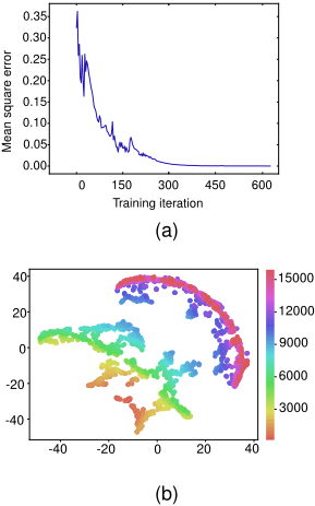
Figure 2a shows the evolution of the training loss over the nominal training period and the rapid convergence of the model (around 300 iterations) towards a negligible value for the reconstruction error. Figure 2b shows the latent representations in a two-dimensional space obtained via the t-SNE algorithm [Maaten and Hinton, 2008]. The time-sequential order of the windows is depicted as the gradual variation of the color space where for example purple corresponds to more recent windows in the monitoring process. Two distinct regions characterize the resulting latent representation space and correspond to a shift of the data distribution. It shows that contiguous signal sequences are projected to a continuous region in the latent space. This is the sign that our model's outputs evolves and adapts to the nominal evolution of the monitored system.
We also evaluate the ability of the continuous learning model to maintain a given regime and that the reconstruction model does not drift on its own over time because of an insufficient nominal training period. Indeed, it is expected that for shorter nominal training periods, the reconstruction model will not be able to consolidate enough its reconstruction capabilities and thus is susceptible to degenerate rapidly in a free-running configuration (where we do not have a mechanism for validating examples) and drift over time which will potentially result in substantial amount of alarms and model replacements. In order to verify capabilities of the continuous learning model, we measure the number of time the controller model is replaced in the case of adaptive control period in different learning configurations. Proposed monitoring model is evaluated using different values for the nominal training period ζ ∈ {200, 500, 1000, 1500, 2000} and Table 1 summarizes obtained results. We notice that regardless of the size of the nominal training period, the reconstruction model is able to maintain a negligible discrepancy over time, measured by the mean square and absolute errors. The same observation can be made regarding the number of alarms triggered by the controller model and the number of time it is replaced.
4.2 Reactivity Assessment
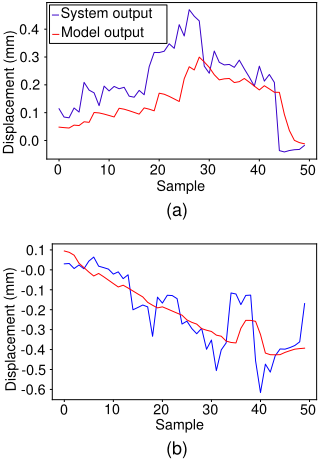
As for the stability of the proposed approach, the reactivity is another important aspect which is evaluated via its ability to be consistent with Equation 7 and to particularly follow abrupt changes of the real system. Figure 3 shows both the system's and our model's outputs within a monitoring window. The analysis shows that the controller model performs well and is able to follow closely the evolution of the system during the considered short windows and in general, its reactivity remains around two time-steps. Even if the obtained results are satisfactory in our case (the residuals in Figure 3a remain within reasonable bounds even during abrupt regime changes), better tuning approach of the α parameter, presented in Equation 7 , can be done to reduce the latency and the discrepancy between the system and our model's outputs.
4.3 Impact of Hyperparameters Optimization
We evaluated more than 600 different architectures which are then analyzed via the functional ANalysis Of VAriance (fANOVA) framework [Hoos and Leyton-Brown, 2014] to assess hyper-parameters relevance and their low-level interactions. Table 2 summarizes the hyper-parameters being optimized along with their corresponding ranges of possible values. Results show that few hyper-parameters have an impact on the performances of the proposed approach. The most influential ones are the number of hidden units, teacher-forcing temperature and the sparsity parameter given by their quantified marginal importance with 0.20185, 0.05866, 0.05954 respectively.
| Hyper-param. (sym) | low | high | prior | marginal importance |
|---|---|---|---|---|
| Learning rate (lr) | 0.001 | 0.1 | log | 0.03677 |
| Weight decay (d) | 0.001 | 0.01 | log | 0.00686 |
| Window size (w) | 10 | 60 | - | 0.02108 |
| Step size (s) | 0.5 | 0.6 | log | 0.00504 |
| Batch size (bs) | 10 | 50 | - | 0.0194 |
| Number of hidden units (nhu) | 64 | 384 | - | 0.20185 |
| Temperature (temp) | 0.2 | 0.5 | log | 0.05866 |
| Sparsity parameter (ρ) | 0.05 | 0.1 | log | 0.05954 |
| Sparsity penalty weight (λ) | 0.5 | 1 | log | 0.01418 |
| Inputs dropout probability (pin) | 0.5 | 1 | log | 0.01621 |
| Outputs dropout probability (pou) | 0.5 | 1 | log | 0.01475 |
| States dropout probability (pst) | 0.5 | 1 | log | 0.00553 |
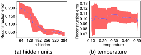
Figure 4 shows the importance of the number of hidden units in the LSTM layers and teacher-forcing temperature on the overall reconstruction performances of the model. As the temperature defines the probability to feed the model with the ground-truth inputs, we expect that the quality of the reconstructions will increase with higher temperature values. Surprisingly, experimental results show that quality remains stable even when the temperature increases. This contrasts with the number of hidden units which has obviously a substantial influence on the reconstruction performances. It shows in particular that larger hidden states, allowed by means of the sparsity criterion that we added, yield better reconstructions. The relatively low importance of most of the hyperparameters compared to the number of hidden units could reflect signs of overfitting. This could stem from the model reconstructing exactly the training data given that we allowed the number of hidden units to exceed inputs dimension. For that matter, the analysis conducted on out-of-sample data using walk-forward validation allows us to check that actually, the model, using the largest number of hidden units, does not suffer from overfitting and is able to reconstruct the validation inputs properly.
5 Conclusion
This paper proposes a two-level LSTM-based autoencoder architecture for monitoring industrial application and reliably account for their evolution over time. We demonstrated significant gains in both reconstruction as well as monitoring performances through Bayesian optimization of the architecture's hyper-parameters. The experimental results on an industrial application prove the effectiveness of the proposed continuous learning model. The success of the proposed approach motivates future work on coupling it with diagnostics capabilities that will open up perspectives for better predictive maintenance.
@inproceedings{ijcai2019p254,
  title     = {Monitoring of a Dynamic System Based on Autoencoders},
  author    = {Osmani, Aomar and Hamidi, Massinissa and Bouhouche, Salah},
  booktitle = {Proceedings of the Twenty-Eighth International Joint Conference on
               Artificial Intelligence, {IJCAI-19}},
  publisher = {International Joint Conferences on Artificial Intelligence Organization},
  editor    = {Sarit Kraus},
  pages     = {1836--1843},
  year      = {2019},
  month     = {8},
  note      = {Main track},
  doi       = {10.24963/ijcai.2019/254},
  url       = {https://doi.org/10.24963/ijcai.2019/254},
}
TY - CPAPER TI - Monitoring of a Dynamic System Based on Autoencoders AU - Osmani, Aomar AU - Hamidi, Massinissa AU - Bouhouche, Salah T2 - Proceedings of the Twenty-Eighth International Joint Conference on Artificial Intelligence, IJCAI-19 PB - International Joint Conferences on Artificial Intelligence Organization PY - 2019 SP - 1836 EP - 1843 DO - 10.24963/ijcai.2019/254 UR - https://doi.org/10.24963/ijcai.2019/254 ER -Copied
Machine-readable versions of this paper, for tools and AI agents:





