
Fast and Accurate Classification with a Multi-Spike Learning Algorithm for Spiking Neurons
Proceedings of the Twenty-Eighth International Joint Conference on Artificial Intelligence. Main track. Pages 1445-1451.
https://doi.org/10.24963/ijcai.2019/200
Keywords
- Humans and AI: Cognitive Modeling
Abstract
The formulation of efficient supervised learning algorithms for spiking neurons is complicated and remains challenging. Most existing learning methods with the precisely firing times of spikes often result in relatively low efficiency and poor robustness to noise. To address these limitations, we propose a simple and effective multi-spike learning rule to train neurons to match their output spike number with a desired one. The proposed method will quickly find a local maximum value (directly related to the embedded feature) as the relevant signal for synaptic updates based on membrane potential trace of a neuron, and constructs an error function defined as the difference between the local maximum membrane potential and the firing threshold. With the presented rule, a single neuron can be trained to learn multi-category tasks, and can successfully mitigate the impact of the input noise and discover embedded features. Experimental results show the proposed algorithm has higher precision, lower computation cost, and better noise robustness than current state-of-the-art learning methods under a wide range of learning tasks.
- [Bohte et al., 2002] Sander M. Bohte, Joost N. Kok, and Han La Poutre. Error-backpropagation in temporally encod- ed networks of spiking neurons. Neurocomputing, 48(1- 4):17-37, 2002.
- [Butts et al., 2007] Daniel A. Butts, Chong Weng, Jianzhong Jin, Chun-I Yeh, Nicholas A. Lesica, Jose-Manuel Alon- so, and Garrett B. Stanley. Temporal precision in the neural code and the timescales of natural vision. Nature, 449(7158):92-95, 2007.
- [Fisher, 1936] Ronald A. Fisher. The use of multiple mea- surements in taxonomic problems. Annals of eugenics, 7(2):179-188, 1936.
- [Florian, 2012] Rȃzvan V. Florian. The chronotron: a neuron that learns to fire temporally precise spike patterns. PLOS ONE, 7(8):e40233, 2012.
- [Gerstner and Kistler, 2002] Wulfram Gerstner and Wern- er M. Kistler. Spiking neuron models: Single neurons, populations, plasticity. Cambridge university press, 2002.
- [Gütig and Sompolinsky, 2006] Robert Gütig and Haim Sompolinsky. The tempotron: a neuron that learns spike timing-based decisions. Nature neuroscience, 9(3):420, 2006.
- [Gütig, 2014] Robert Gütig. To spike, or when to spike? Current opinion in neurobiology, 25:134-139, 2014.
- [Gütig, 2016] Robert Gütig. Spiking neurons can discover predictive features by aggregate-label learning. Science, 351(6277):aab4113, 2016.
- [Miao et al., 2018] Yu Miao, Huajin Tang, and Gang Pan. A supervised multi-spike learning algorithm for spiking neu- ral networks. International Joint Conference on Neural Networks, pages 1-7, 2018.
- [Nakamura et al., 2000] Satoshi Nakamura, Kazuo Hiyane, Futoshi Asano, Takanobu Nishiura, and Takeshi Yamada. Acoustical sound database in real environments for sound scene understanding and hands-free speech recognition. In Language Resources and Evaluation Conference, 2000.
- [Orchard et al., 2015] Garrick Orchard, Cedric Meyer, Ralph Etienne-Cummings, Christoph Posch, Nitish Thakor, and Ryad Benosman. Hfirst: a temporal approach to object recognition. IEEE transactions on pattern analysis and machine intelligence, 37(10):2028-2040, 2015.
- [Pérez-Carrasco et al., 2013] José A. Pérez-Carrasco, Bo Zhao, Carmen Serrano, Begona Acha, Teresa Serrano-Gotarredona, Shouchun Chen, and Bernabé Linares-Barranco. Mapping from frame-driven to frame- free event-driven vision systems by low-rate rate coding and coincidence processing-application to feedforward convnets. IEEE transactions on pattern analysis and machine intelligence, 35(11):2706-2719, 2013.
- [Ponulak and Kasiński, 2010] Filip Ponulak and Andrze- j Kasiński. Supervised learning in spiking neural networks with resume: sequence learning, classification, and spike shifting. Neural Computation, 22(2):467-510, 2010.
- [Qi et al., 2018] Yu Qi, Jiangrong Shen, Yueming Wang, Huajin Tang, Hang Yu, Zhaohui Wu, and Gang Pan. Joint- ly learning network connections and link weights in spik- ing neural networks. pages 1597-1603. International Joint Conferences on Artificial Intelligence, 2018. IJCAI
- [Song et al., 2000] Sen Song, Kenneth D. Miller, and Lar- ry F. Abbott. Competitive hebbian learning through spike-timing-dependent synaptic plasticity. Nature neuro- science, 3(9):919-926, 2000.
- [VanRullen et al., 2005] Rufin VanRullen, Rudy Guyon- neau, and Simon J. Thorpe. Spike times make sense. Trends in neurosciences, 28(1):1-4, 2005.
- [Xiao et al., 2018] Rong Xiao, Huajin Tang, Pengjie Gu, and Xiaoliang Xu. Spike-based encoding and learning of spec- trum features for robust sound recognition. Neurocomput- ing, 2018.
- [Xu et al., 2018] Qi Xu, Yu Qi, Hang Yu, Jiangrong Shen, Huajin Tang, and Gang Pan. Csnn: An augmented spiking based framework with perceptron-inception. pages 1646- 1652. International Joint Conferences on Artificial Intelli- gence, 2018. IJCAI
- [Yu et al., 2013] Qiang Yu, Huajin Tang, Kay C. Tan, and Haizhou Li. Precise-spike-driven synaptic plasticity: Learning hetero-association of spatiotemporal spike pat- terns. PLOS ONE, 8(11):e78318, 2013.
- [Yu et al., 2018a] Qiang Yu, Haizhou Li, and Kay C. Tan. Spike timing or rate? neurons learn to make decisions for both through threshold-driven plasticity. IEEE transac- tions on cybernetics, (99):1-12, 2018.
- [Yu et al., 2018b] Qiang Yu, Longbiao Wang, and Jianwu Dang. Efficient multi-spike learning with tempotron-like ltp and psd-like ltd. In International Conference on Neural Information Processing, pages 545-554, 2018.
- [Zhang et al., 2018] Malu Zhang, Hong Qu, Ammar Be- latreche, Yi Chen, and Zhang Yi. A highly effective and robust membrane potential-driven supervised learning method for spiking neurons. IEEE transactions on neural networks and learning systems, (99):1-15, 2018.
- [Zhao et al., 2014] Bo Zhao, Ruoxi Ding, Shoushun Chen, Bernabe Linares-Barranco, and Huajin Tang. Feedforward categorization on aer motion events using cortex-like fea- tures in a spiking neural network. IEEE transactions on neural networks and learning systems, 26(9):1963-1978, 2014.
References were extracted automatically from the PDF and may contain errors.
Full text extracted automatically from the PDF; figures, tables and equations may differ. The PDF is the version of record.
1 Introduction
Spiking neural networks (SNNs) [Gerstner and Kistler, 2002] simulate the fundamental mechanism of our brain and provide greater computational power and more biological realism [VanRullen et al., 2005; Butts et al., 2007; G¨utig, 2014]. The basic computation model of single neuron is the transformation of incoming spike trains into appropriate spike output. How could spiking neurons learn to make decisions on spike patterns? Many different learning methods have been proposed by adjusting the synaptic efficacy of neurons to generate desired sequences of spikes [Song et al., 2000; Florian, 2012; Qi et al., 2018; Xu et al., 2018].
Among the existing spike-based learning algorithms, tempotron [G¨utig and Sompolinsky, 2006] has only two output states in response to input patterns: firing or not firing, and thus it is efficient for binary classification tasks. However, the behavior of neuron with tempotron constrains its ability on temporal output structure. To address the limitations, researchers have proposed different learning algorithms to train the spiking neurons to produce a precise-timing spike train at the desired firing time, such as ReSuMe [Ponulak and Kasi´nski, 2010] and PSD [Yu et al., 2013]. ReSuMe rule is capable of performing spike-timing-based learning precisely by exploiting STDP and anti- STDP processes based on the Widrow-Hoff (WH) rule. PSD rule can emit multiple spikes at the desired firing time, which is based on the WH rule and the exponential kernel. Neurons with these rules are suitable for processing different classes due to different output spike timing could be associated with different classes. However, the internal mechanisms about how to construct such a precise spike sequence are still unclear in biological neurons. And when faced real-world problems, they are relatively limited mainly due to inherent computational complexity.
∗Corresponding author: huajin.tang@gmail.com
Recently, a new membrane potential-driven multi-spike tempotron (MST) rule [G¨utig, 2016] has been developed to train neurons to fire desired number of spikes, which empowers them to discover sensory features embedded in a complex background activity. Inspired by this work, two different multi-spike learning rules (TDP1 and TDP2) [Yu et al., 2018a] have been developed, in an attempt to improve the learning efficiency in spiking neurons. [Yu et al., 2018a] introduces a simple alternative, the linear assumption for threshold crossing [Bohte et al., 2002] to complete the computation, and provides analytical proofs on convergence and stability on such multi-spike learning rules. In later work, Miao et al. [Miao et al., 2018] propose another supervised multi-spike learning algorithm. It modifies synaptic weights and makes the neuron's output reach the desired number by using local maximum point. However, a common disadvantage of the methods is computationally intensive, resulting in relatively low learning efficiency, thus can't meet the requirements of the real-time applications.
To address this issue, preliminary attempt has demonstrated great improvement on efficiency by combining both the Tempotron and PSD rules [Yu et al., 2018b]. In this paper, we further propose a simple and novel multi-spike learning rule for spiking neurons, which can quickly find a suitable local maximum value as the relevant signal for synaptic updates, based on the membrane potential trace of a neuron rather than the STS function. This value is closest to the threshold and can make the neuron's output reach the desired number as fast as possible. We employ an error function defined as the difference between the local maximum membrane potential of output neuron and its firing threshold, thus allows the application of gradient descent to optimize the synaptic weights. Besides, the learning efficiency of the method is significantly improved through the introduction of event-driven manner. Various properties of the proposed learning rule are investigated through extensive experimental analysis. Experimental results have shown the advantages of the proposed algorithm under a wide range of learning tasks.
2 Event-Driven LearningMethod
2.1 NeuronModel
The leaky integrate-and-fire (LIF) neuron model [Gerstner and Kistler, 2002] is introduced due to its simplicity and computational effectivity. The neuron's membrane potential V (t) is given by integrating its synaptic currents from N afferent neurons:
where tji is the arrival time of the j-th presynaptic spike of the i-th afferent and tjs denotes the time of the j-th output spike elicited in the postsynaptic compartment. Each afferent spike contributes a postsynaptic potential (PSP), whose peak amplitude is determined by the afferent's synaptic efficacy wi and the kernel K, which is defined as:
where τm and τs are the membrane time constants of the membrane potential and synaptic currents respectively, and τm/τs = 4. V0 is a normalization factor. When V (t) crosses the firing threshold ϑ, the neuron will emit an output spike, and the membrane potential is reset to the potential Vr.
2.2 Event-Driven Computation
For the event-based manner, the spike is calculated one after another in an ordered time sequence [Yu et al., 2018a]. We define the voltage of the k-th input spike:
The states of Ekm, Ek s and Ek are expressed recursively as:
2.3 Learning Rule
In [G¨utig, 2016], STS function was defined to learn the relation between the number of output spikes k and the threshold θ∗ k . Within each iteration, the θ∗ was recalculated for updating weights. Gutig employed the numerical approximations with a complex recursive computation to solve the derivative of θ∗ . Although Yu et al. [Yu et al., 2018a] simplified computation by a linear approximation for threshold crossing to get approximations for the derivative of θ∗ , the necessary computation of STS function for every synaptic update was still time consuming. Miao et al. [Miao et al., 2018] further introduced local maximum points under an infinite threshold to find θ∗ for a given θ. The common disadvantage was that the method still introduced additional membrane potential traces. Meanwhile, it brought a complex computation problem because of time-based simulation mechanism thus resulting in relatively low learning efficiency. We implement a novel learning rule with the simplest form of membrane potential traces where only the actual membrane potential (easily accessible) is considered as the relevant signal for synaptic updates. There is no requirement to calculate additional membrane potential traces. Thus θ∗ can be quickly obtained as the point of modifiable weight (see Table 1).
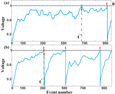
Considering all event points [t1, t2, ..., tn], we obtain the membrane potential traces as shown in Figure 1. Firstly, we define V (tk-1) as the membrane voltage of tk-1. When the k-th spike occurs, the membrane voltage of the neuron will change denoted as V (tk) = V (tk-1) + ∆V . If V (tk) in
| Method | STS function | Calculate a gradient of θ∗ | Output spike | Learning rule | Driving mode |
|---|---|---|---|---|---|
| tempotron | No | No | Binary output | Gradient-based WH rule | Time-based |
| PSD | No | No | Precise-timing spike | Time-based | |
| ReSuMe | No | No | Precise-timing spike | WH rule + STDP | Time-based |
| MST | Yes | Recursive approach | Spike number | Gradient-based | Event-based |
| TDP1, TDP2 | Yes | Linear function | Spike number | Gradient-based | Event-based |
| Miao's method | No | Local maximum point | Spike number | Gradient-based | Time-based |
| This work | No | Local maximum point | Spike number | Gradient-based | Event-based |
Algorithm 1 The Algorithm of Multi-Spike Learning
Input: Weight vector W, input spikes P Output: Output spike number na
1: procedure MULTI-SPIKE LEARNING 2: for each iteration do 3: for each input spike with time tk in P do 4: Compute Potential with Equation 4,5 5: if V (tk) ≥ ϑ then 6: Generate an output spike, na ← na + 1 7: D+ ← Dk by Equation 6 8: Ek ← Ek + ϑ 9: else 10: if V (tk) is local maximum value then 11: D- ← Dk by Equation 7 12: end if 13: end if 14: end for 15: if na > nd then 16: Find max D+ as D∗ 17: Compute ∆wk by Equation 14 18: end if 19: if na < nd then 20: Find min D- as D∗ 21: Compute ∆wk by Equation 14 22: end if 23: Update Weight W ← W + ∆wk 24: end for; 25: end procedureAccording to the chain rule, the second term is defined as:
It can be computed by introducing the linear assumption [Yu et al., 2018a]. The last term is a vanishing part since V ∗ (t∗ ) is either a local maximum with ∂V ∗ (t∗ )/∂t∗ = 0 or t∗ is the time of an inhibitory input spike whose arrival time does not depend on wi. For further simplifying the method, we only take consideration of partial derivatives with respect to wi (ignoring the second term, refer to TDP2) as:
the tk is a local maximum, we define Dk = (θ - V (tk)) = θ - V (tk-1) -∆V to denote the difference between the desired value to cross θ and actual changed value for the k-th input spike. A difference set D based on all the local maximum value of membrane potential is collected. With a given threshold ϑ, we separate the D into two subsets: D+ and D-.
Based on the existence of D, we can get these event points corresponding to the local maximum value. Our final goal is to find a suitable event point t∗ which aims to modify synaptic weights and makes the neuron's output reach the desired number as fast as possible. Thus we change the neuron's output spike number by modifying weights with respect to the local maximum V ∗ (t∗ ) closest to the threshold. Comparing na and nd, there are two cases:
1)na < nd : To make na equal nd, we assume the t∗ is the event point which corresponds to the minimum value of the difference in D-. It is given as D∗ = min{D-}(see Figure 1'+'). For the event point at t∗ , the value of the neuron membrane potential is expected to cross the firing threshold to fire a spike. The cost function is constructed as follows:
2)na > nd : We define the t∗ is the event point which corresponds to the maximum value of the difference in D+. It is given as D∗ = max{D+}(see Figure 1'×'). To avoid the occurrence of undesired output spikes, the membrane potential is required to remain below the neuron firing threshold. The cost function is defined as:
This rule performs gradient-descent rule as:
η > 0 is the learning rate. The derivative of c with respect to weight wi is expressed as:
where the previous output spike times tjs < t∗ , j ∈ {1, 2, ...,m}. The first term can be expressed as:
3 Experimental Setup
There are N afferent neurons, and each afferent neuron emits a spiking train with a Poisson rate of rin Hz over a time interval T. The default parameters used in the following experiments are set as N = 500, T = 0.5 s. The initial synaptic weight is selected randomly from a Gaussian distribution with a mean value of 0.01 and a standard deviation of 0.01. The spike threshold ϑ = 1, and the reset potential Vr = 0. We set the parameters η = 0.0001, τm = 20 ms, and τs = 5 ms. Parameters different from the default setups will be stated otherwise. All data are averaged over ten independent runs.
3.1 Effects of Initial Setups
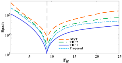
We show the dependence of the neuron's learning speed and initial output spikes on the different firing rate rin. The input spike train of each input neuron is generated by a Poisson process ranging from 1 Hz to 25 Hz. The learning rate is scaled as η·rin/r0 in with r0 in = 4 Hz. The desired output spike number is set as nd out = 20. During the training process, the closer the distance between the actual and the desired output number, the less the training epochs needed to complete convergence. Besides, the training epoch increases exponentially with the distance between the initial and the desired output number increases. Figure 2 shows that our algorithm is superior to MST and TDP2, and achieves an approximate performance with the TDP1 in training epochs. To further explore the
| Firing rate | This work | MST | TDP1 | TDP2 |
|---|---|---|---|---|
| 5 | 0.013 | 0.037 | 0.020 | 0.018 |
| 10 | 0.015 | 0.068 | 0.052 | 0.039 |
| 15 | 0.014 | 0.119 | 0.098 | 0.070 |
| 20 | 0.016 | 0.200 | 0.165 | 0.123 |
| 25 | 0.017 | 0.270 | 0.240 | 0.180 |
learning efficiency, the training time of one epoch is tested at various firing rates. Each spike train is generated by a Poisson process with firing rate ranging from 5 Hz to 25 Hz. Table 2 indicates that the higher the firing rate, the more time required for the other three algorithms to complete one training epoch. That is because of more input spikes required to be trained.
However, our algorithm consumes less time than traditional ones and maintains a relatively consistent training time at various firing rates.
3.2 Effects of Parameters
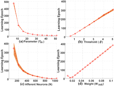
Here, we explore the influence of the parameter τm, the threshold θ, the initial mean weight Winit, and the number of afferent neurons N on the learning epoch. The neuron is trained with τm = 20, N = 500, θ = 1 and Winit = 0.01.
Figure 3(a) shows the learning epoch for different τm. Different values of τm will have some different influence on the convergent speed. A higher value leads to less learning epochs, while when it above 20, this change is not obvious. Fig. 3(b) shows the learning epoch for different θ. It suggests that the threshold directly affects the speed of convergence. In real-world applications, θ can be set to different values according to different requirements. Figure 3(c) depicts the learning epoch for different N. In the beginning, more input neurons lead to less learning epochs, while when it above 500, this change is not obvious. This is mainly because more input neurons make more sparse representation of the input patterns, which are easier to be trained because there is less interference between different patterns. Figure 3(d) displays the learning epoch for different Winit. It shows the fastest learning speed appears at the point of the best matching initial output to the desired one (like Winit = 0.015).
3.3 Robustness to Noise
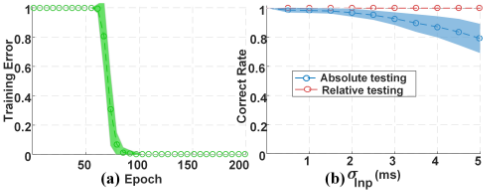
The reliability of the neuron's response could be influenced by different noise. Here, ten spike patterns without noise are randomly generated by using precise timing encoding. We fix these patterns as the training templates. The neuron is trained for 200 epochs with 10 desired spike number. After training, a Gaussian jitter with a mean = 0 and standard deviation σInp ∈ [0, 5] is used to generate the noise patterns. Each template is used to construct 20 testing patterns. For each noise level, there are a total number of 200 noise patterns for testing. In Figure 4(a), the output stabilizes quickly and can exactly converge to the desired spike number (about 80 training epochs). In Figure 4(b), two testing scenarios are considered, i.e., absolute and relative testing. With the absolute testing, the input pattern will be regarded as being correctly classified, only if the output spike number equals the desired spike. For the relative testing, the incoming pattern will be deemed to be successfully classified if the output spike number belongs to the pre-defined range with r = 1. In the relative testing, the classification accuracy is 100% and remains unchanged. In the absolute testing, the accuracy will decrease with the increasing noise intensity. But our method still can successfully reproduce the desired spike number with relatively high accuracy (90%) even when the noise strength is 3.
3.4 Learning Predictive Clues
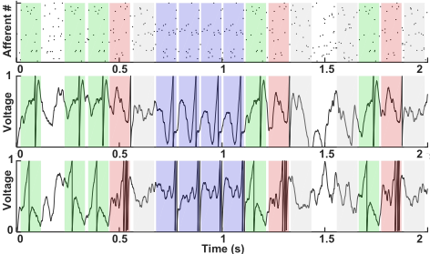
We demonstrate the ability of our algorithm for solving the challenging task of the temporal credit-assignment problem as mentioned in [G¨utig, 2016; Yu et al., 2018a]. Similar to the task in [Yu et al., 2018a], six activity patterns with the background firing statistics are randomly generated, in which a random half of the activity patterns are assigned as feature patterns while another half as distractors. For each activity pattern, there are 500 afferent neurons and one output neuron.
Each afferent neuron emits a spiking train with a Poisson rate of rin = 4 Hz over a time interval T = 2 s. The output neuron is trained to produce a specific number of spikes when a feature pattern is presented, while keeping silence when a pattern from the distractors or background activities is presented. The total desired output spike number nd out in response to feature patterns will be nd out = ∑pi=1 cidi where ci is the occurrence number of the i-th feature pattern and di is the desired output spike number in response to the i-th feature pattern. p is the total number of feature patterns, which is set to 3. The values of di for the 3 feature patterns are set as {1, 1, 1} and {1, 2, 3}. Figure 5 show that the single neuron can successfully perform two challenging credit-assignment task.
4 Experimental Results
We investigate the capability of our algorithm over real classification tasks. Each neuron is trained to produce nd out = 10 spikes when a pattern from the assigned class is presented while keeping silence when patterns from other classes are presented. For each trial, a momentum heuristic method is introduced to accelerate learning [G¨utig and Sompolinsky, 2006]. The updating of current synaptic weight ∆wcurr i consists of the precious synaptic change ∆pre wi and the correction given by the learning rule ∆wi, which is constructed as follows: ∆wcurr i =∆wi+µ∆pre wi , µ = 0.9. For the testing result, the responses of all neurons to each pattern are tested. The incoming pattern will be regarded as belonging to the corresponding class which the neuron represents when the output spike number emitted by the neuron is the most.
4.1 Dataset Description
- Iris [Fisher, 1936]. It contains 3 classes with 4 attributes. Each input feature is encoded by 6 neurons with Gaussian receptive fields. The total time duration of the input spatiotemporal pattern is set to T = 10 ms. We choose 50% for training and the others for testing.
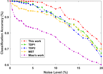
- OCR [Yu et al., 2013]. This includes images of digits 09. We introduce noise as described in [Yu et al., 2013]. There are 100 samples for training. For each noise level of 0-20%, 100 noise patterns are generated for testing.
- AER Poker Card [P´erez-Carrasco et al., 2013]. This contains the event stream of 4 card symbols, each with 10 examples. We choose 50% data for training and the others for testing. We execute feature extraction with event-based gabor filter [Orchard et al., 2015].
- RWCP [Nakamura et al., 2000]. We select 10 sound classes with 16 kHz sampling rate. The LTF-SNN feature encoding method [Xiao et al., 2018] is used. For each class, 20 clean classes are used for training. After training, the babble noise is added to 20 testing data with clean, 20, 10, and 0 signal-to-noise ratio (SNR).
| Dataset | MST | TDP1 / TDP2 | Miao's work | This work | |||||||||||
|---|---|---|---|---|---|---|---|---|---|---|---|---|---|---|---|
| Accuracy | Epoch | Time(s) | Accuracy | Epoch | Time(s) | Accuracy | Epoch | Time(s) | Accuracy | Epoch | Time(s) | ||||
| Iris | 96.30 | 350 | 20.1 | 96.40 | / 96.50 | 350 | / 350 | 17.3 | / 15.9 | 60.00 | 300 | 7.5 | 96.30 | 350 | 4.5 |
| OCR | 88.00 | 500 | 791 | 91.00 | / 90.00 | 274 / | 500 | 260 | / 325 | 78.23 | 500 | 5671 | 93.00 | 247 | 29 |
| Poker Card | 100.00 | 12 | 30 | 100.00 | / 100.00 | 13 / | 14 | 17 | / 14 | 100.00 | 14 | 10 | 100.00 | 10 | 2.1 |
| Noise | This work | MST | TDP1 | TDP2 | Miao's work | Tempotron | ReSuMe | R-MemPo-Learn |
|---|---|---|---|---|---|---|---|---|
| Clean | 100.00 | 100.00 | 100.00 | 100.00 | 99.99 | 100.00 | 94.80 | 97.80 |
| 20dB | 100.00 | 100.00 | 100.00 | 100.00 | 99.98 | 100.00 | 92.50 | 97.10 |
| 10dB | 100.00 | 100.00 | 100.00 | 99.00 | 99.26 | 98.00 | 90.60 | 96.40 |
| 0dB | 92.50 | 91.00 | 90.50 | 88.60 | 88.41 | 90.50 | 84.40 | 91.10 |
| Average | 98.13 | 97.75 | 97.63 | 96.90 | 96.91 | 97.13 | 90.58 | 95.60 |
| Total time (s) | 16 | 193 | 138 | 129 | 482 | / | / | / |
4.3 Discussion
In time-based simulation, time steps are T . At each time step, we recalculate the postsynaptic potential of input spikes before current time. The time complexity is O(T). In eventbased simulation, we update the status only when there is an incoming spike. The time complexity is O(N) where N is the number of input spikes and N ≪ T. In calculating each incoming spike, it involves 8 multiplication and 7 addition/subtraction/comparison (refer to [Zhao et al., 2014]).
- Number of multiplication=8 × N
- Number of addition/subtraction/comparison=7 × N
For STS function, it learns the relation between the number of output spikes k and the neuron's threshold θ∗ k (k varies from 1 to M). For each k in M, the operations as mentioned above are repeated again.
- Number of multiplication=8 × N × M
- Number of addition/subtraction/comparison=7 ×N ×M We only execute N additional comparisons for all incoming spike, thus simplify the membrane potential calculation.
- Number of multiplication=8 × N
- Number of addition/subtraction/comparison=8 × N.
5 Conclusion
We propose a simple and effective multi-spike learning rule which is used to train neurons to fire the desired number of output spikes. The output spike number is changed by modifying the synaptic weights of the local maximum point based on membrane potential trace of a neuron rather than the sophisticated STS method [G¨utig, 2016]. This operation simplifies the membrane potential calculation. Experimental results show that our method is capable of recognizing objects correctly with performance comparable to that of current benchmark algorithms for a wide spectrum of datasets.
Acknowledgments
This work was supported by the National Natural Science Foundation of China under grant numbers 61673283 and 61773271.
4.2 Results
Table 3 and Table 4 show the classification accuracy and the learning time of different methods. Compared with the traditional classifiers, our algorithm spends less time to complete training and achieves better recognition performance especially for the data with noise. We investigate the robustness on OCR dataset as shown in Figure 6. For 5 different classifiers, the classification accuracy remains high when the noise level is low and will decrease gradually with the increasing noise level. Our method obtains the highest average accuracy of 93% even when the image is severely damaged by 20% noise level (see Table 3). The performance comparison at each noise level for RWCP dataset is presented in Table 4. The proposed method performs well for each of the noise conditions, achieving a relatively high accuracy of 98.13%. The classification accuracy of TDP2 and ReSuMe is high under clean or low-noise environment, while the performance decreases dramatically in 0dB SNR condition. It means the robustness of the proposed method is better than the other investigated spike-based methods (Tempotron, ReSuMe, and R-MemPo-Learn [Xiao et al., 2018; Zhang et al., 2018]). Besides, Table 4 shows that our method is obviously superior in training time, which only needs 16s, much less than other algorithms.
@inproceedings{ijcai2019p200,
  title     = {Fast and Accurate Classification with a Multi-Spike Learning Algorithm for Spiking Neurons},
  author    = {Xiao, Rong and Yu, Qiang and Yan, Rui and Tang, Huajin},
  booktitle = {Proceedings of the Twenty-Eighth International Joint Conference on
               Artificial Intelligence, {IJCAI-19}},
  publisher = {International Joint Conferences on Artificial Intelligence Organization},
  editor    = {Sarit Kraus},
  pages     = {1445--1451},
  year      = {2019},
  month     = {8},
  note      = {Main track},
  doi       = {10.24963/ijcai.2019/200},
  url       = {https://doi.org/10.24963/ijcai.2019/200},
}
TY - CPAPER TI - Fast and Accurate Classification with a Multi-Spike Learning Algorithm for Spiking Neurons AU - Xiao, Rong AU - Yu, Qiang AU - Yan, Rui AU - Tang, Huajin T2 - Proceedings of the Twenty-Eighth International Joint Conference on Artificial Intelligence, IJCAI-19 PB - International Joint Conferences on Artificial Intelligence Organization PY - 2019 SP - 1445 EP - 1451 DO - 10.24963/ijcai.2019/200 UR - https://doi.org/10.24963/ijcai.2019/200 ER -Copied
Machine-readable versions of this paper, for tools and AI agents:





