
An Evolution Strategy with Progressive Episode Lengths for Playing Games
Proceedings of the Twenty-Eighth International Joint Conference on Artificial Intelligence. Main track. Pages 1234-1240.
https://doi.org/10.24963/ijcai.2019/172
Keywords
- Heuristic Search and Game Playing: Game Playing and Machine Learning
- Machine Learning Applications: Game Playing
Abstract
Recently, Evolution Strategies (ES) have been successfully applied to solve problems commonly addressed by reinforcement learning (RL). Due to the simplicity of ES approaches, their runtime is often dominated by the RL-task at hand (e.g., playing a game). In this work, we introduce Progressive Episode Lengths (PEL) as a new technique and incorporate it with ES. The main objective is to allow the agent to play short and easy tasks with limited lengths, and then use the gained knowledge to further solve long and hard tasks with progressive lengths. Hence allowing the agent to perform many function evaluations and find a good solution for short time horizons before adapting the strategy to tackle larger time horizons. We evaluated PEL on a subset of Atari games from OpenAI Gym, showing that it can substantially improve the optimization speed, stability and final score of canonical ES. Specifically, we show average improvements of 80% (32%) after 2 hours (10 hours) compared to canonical ES.
- [Alvernaz and Togelius, 2017] S. Alvernaz and J. Togelius. Autoencoder-augmented neuroevolution for visual doom playing. In Proc. of IEEE CIG, pages 1-8, 2017.
- [Bengio et al., 2009] Y. Bengio, J. Louradour, R. Collobert, and J. Weston. Curriculum learning. In Proc. of ICML, pages 41-48, 2009.
- [Brockman et al., 2016] G. Brockman, V. Cheung, L. Pet- tersson, J. Schneider, J. Schulman, J. Tang, and W. Zaremba. Openai gym. arXiv:1606.01540 [cs.LG], 2016.
- [Chrabaszcz et al., 2018] P. Chrabaszcz, I. Loshchilov, and F. Hutter. Back to basics: Benchmarking canonical evolu- tion strategies for playing atari. In Proc. of IJCAI, pages 1419-1426, 2018. IJCAI
- [Clevert et al., 2016] D.-A. Clevert, T. Unterthiner, and S. Hochreiter. Fast and accurate deep network learning by exponential linear units (elus). In Proc. of ICLR, 2016.
- [Conti et al., 2018] E. Conti, V. Madhavan, F. Such, J. Lehman, K. Stanley, and J. Clune. Improving ex- ploration in evolution strategies for deep reinforcement learning via a population of novelty-seeking agents. arXiv:1712.06560 [cs.AI], 2018.
- [Cuccu et al., 2018] G. Cuccu, J. Togelius, and P. Cudre- Mauroux. Evolutionary generative adversarial networks. arXiv:1803.00657 [cs.LG], 2018.
- [Falkner et al., 2018] S. Falkner, A. Klein, and F. Hutter. BOHB: robust and efficient hyperparameter optimization at scale. In Proc. of ICML, pages 1436-1445, 2018.
- [Jiang et al., 2015] L. Jiang, D. Meng, Q. Zhao, S. Shan, and A. Hauptmann. Self-paced curriculum learning. In Proc. of AAAI, pages 2694-2700, 2015.
- [Karnin et al., 2013] Z. Karnin, T. Koren, and O. Somekh. Almost optimal exploration in multi-armed bandits. In Proc. of ICML, pages 1238-1246, 2013.
- [LaPorte et al., 2015] G. LaPorte, J. Branke, and C.-H. Chen. Adaptive parent population sizing in evolution strategies. Evolutionary Computation, 23:397-420, 2015.
- [Li et al., 2017] L. Li, K. Jamieson, G. DeSalvo, A. Ros- tamizadeh, and A. Talwalkar. Hyperband: A novel bandit- based approach to hyperparameter optimization. Journal of Machine Learning Research, 18:185:1-185:52, 2017.
- [Miller et al., 1989] G. Miller, P. Todd, and S. Hegde. De- signing neural networks using genetic algorithms. In Proc. of ICGA, pages 379-384, 1989.
- [Mnih et al., 2013] V. Mnih, K. Kavukcuoglu, D. Silver, A. Graves, I. Antonoglou, D. Wierstra, and M. Ried- miller. Playing atari with deep reinforcement learning. arXiv:1312.5602 [cs.LG], 2013.
- [Mnih et al., 2015] V. Mnih, K. Kavukcuoglu, D. Silver, A. Rusu, J. Veness, M. Bellemare, A. Graves, M. Ried- miller, A. Fidjeland, G. Ostrovski, S. Petersen, C. Beat- tie, A. Sadik, I. Antonoglou, H. King, D. Kumaran, D. Wierstra, S. Legg, and D. Hassabis. Human-level control through deep reinforcement learning. Nature, 518(7540):529-533, 2015.
- [Narvekar, 2017] S. Narvekar. Curriculum learning in rein- forcement learning. In Proc. of IJCAI, pages 5195-5196, 2017. IJCAI
- [Poulsen et al., 2017] A. Poulsen, M. Thorhauge, M. Funch, and S. Risi. DLNE: A hybridization of deep learning and neuroevolution for visual control. In Proc. of IEEE CIG, pages 256-263, 2017.
- [Real et al., 2017] E. Real, S. Moore, A. Selle, S. Saxena, Y. Suematsu, J. Tan, Q. Le, and A. Kurakin. Large-scale evolution of image classifiers. In Proc. of ICML, pages 2902-2911, 2017.
- [Rechenberg, 1973] I. Rechenberg. Evolutionsstrategie opti- mierung technisher systeme nach prinzipien der biologis- chen evolution. PhD thesis, Frommann-Holzboog, 1973.
- [Risi and Togelius, 2017] S. Risi and J. Togelius. Neuroevo- lution in games: State of the art and open challenges. IEEE Trans. Comput. Intellig. and AI in Games, 9(1):25- 41, 2017.
- [Salimans et al., 2016] T. Salimans, I. Goodfellow, W. Zaremba, V. Cheung, A. Radford, and X. Chen. Improved techniques for training gans. In Pros. of NIPS, 2016.
- [Salimans et al., 2017] T. Salimans, J. Ho, X. Chen, and S. Sidor amd I. Sutskever. Evolution strategies as a scalable alternative to reinforcement learning. arXiv:1703.03864 [stat.ML], 2017.
- [Schulman et al., 2017] J. Schulman, S. Levine, P. Moritz, M. Jordan, and P. Abbeel. Trust region policy optimiza- tion. arXiv:1502.05477 [cs.LG], 2017.
- [Silver et al., 2017] D. Silver, J. Schrittwieser, K. Simonyan, I. Antonoglou, A. Huang, A. Guez, T. Hubert, L. Baker, M. Lai, A. Bolton, Y. Chen, T. Lillicrap, F. Hui, L. Sifre, G. Driessche, T. Graepel, and Demis Hassabis. Master- ing the game of go without human knowledge. Nature, 550:354-359, 2017.
- [Such et al., 2017] F. Such, V. Madhavan, E. Conti, J. Lehman, K. Stanley, and J. Clune. Deep neuroevolu- tion: Genetic algorithms are a competitive alternative for training deep neural networks for reinforcement learning. CoRR, abs/1712.06567, 2017.
- [Swersky et al., 2013] K. Swersky, J. Snoek, and R. Adams. Multi-task bayesian optimization. In Proc. of NIPS, pages 2004-2012, 2013.
- [Wierstra et al., 2014] D. Wierstra, T. Schaul, T. Glasmach- ers, Y. Sun, J. Peters, and J. Schmidhuber. Natural evolu- tion strategies. JMLR, 15:949-980, 2014.
References were extracted automatically from the PDF and may contain errors.
Full text extracted automatically from the PDF; figures, tables and equations may differ. The PDF is the version of record.
1 Introduction
In reinforcement learning (RL), an agent learns how to solve a given task by interacting with its environment. Recent advances using deep policy networks have successfully addressed problems previously considered to be unsolvable, including surpassing the level of a world champion Go Player [Silver et al., 2017] and playing well a large collection of Atari games [Mnih et al., 2015].
Recently, evolution strategy (ES) showed surprisingly good performance as an alternative approach to deep RLalgorithms for playing Atari games [Salimans et al., 2017; Conti et al., 2018; Chrabaszcz et al., 2018]. The ES directly optimizes the weights of deep policy networks encoding a mapping from states to actions. Thus, an ES approach for RL consists of optimizing a population of policies in the spaces of potentially millions of network weights. The advantages of ES compared to gradient-based optimizers are that (i) ES is a gradient-free black-box approach which is able to optimize non-differentiable functions and more importantly,
- (ii) ES can be efficiently parallelized resulting in short optimization time compared to sequential optimizers and many deep RL-algorithms [Salimans et al., 2017].
Whereas the advantages of ES are intriguing, ES has some drawbacks similarly to the ones observed in RL. Although ES uses parallel resources efficiently, ES still has to evaluate many episodes and thus needs a lot of CPU time, e.g., Chrabaszcz et al. [2018] used 4000 CPU hours for a single ES run. Nevertheless, ES approaches are often trapped in local optima shown by better policies found by RL-approaches or even random search on some games [Such et al., 2017].
In this work, we aim to advance the state-of-the-art of ES for RL-problems and propose a new algorithm, evaluated on Atari games from OpenAI. The contributions of this work are:
- We introduce a novel technique which we dub Progressive Episode Lengths (PEL) and show how to incorporate it into canonical ES [Rechenberg, 1973; Chrabaszcz et al., 2018]. The underlying idea is to allow an agent to play short and easy tasks first, and then use the gained knowledge to further solve longer and harder tasks, similar as in transfer learning and curriculum learning.
- We demonstrate the use of different time and episode schedulers in PEL, controlling the maximal episode length for a given time frame.
- On a set of OpenAI Gym games, we show that ES is often able to learn a policy on short episodes and transfer this policy to longer episodes.
- We study the empirical performance of PEL approach with different time schedulers and show that after 2 (10) hours of training, the agent is able to play the game with an average improvement of 80% (32%) compared to the use of canonical ES without PEL.
2 RelatedWork
The foundation of ES approaches are built upon the early work of Rechenberg [1973]. In recent years, ES has been proposed as an alternative approach to RL algorithms. Salimans et al. [2017] showed that using a natural ES [Wierstra et al., 2014] can achieve comparable results in a few hours compared to sequential RL methods (e.g., [Mnih et al., 2015; Schulman et al., 2017]). Following Salimans's work, Chrabaszcz et al. [2018] showed that an even simpler canonical ES can achieve better results.
Conti et al. [2018] proposed a method that improves the exploration of ES by introducing novelty seeking. This technique tries to avoid local optima and induce exploration by completely ignoring the reward function and selecting agents which perform new behaviors. The results show that the proposed algorithm can learn to play Atari games and solve MuJoCo 3D humanoid tasks even when completely ignoring the reward input. LaPorte et al. [2015] proposed an adaptive parent population method in ES, aiming to adapt the parent population size which maximizes the final results.
ES approaches are applied in various disciplines and have been incorporated in various fields in machine learning. Cuccu et al. [2018] incorporated an ES approach with compact state representation. Using vector quantization and sparse coding, the used neural network containing only 6 to 18 neurons is capable of playing Atari games. Miller et al. [1989] used ES to design neural networks, leading to a modern ES for neural architecture search (e.g., [Real et al., 2017]) and neuroevolution for playing games [Risi and Togelius, 2017]. Furthermore, Alvernaz and Togelius [2017] and Poulsen et al. [2017] combined gradient-based RLapproaches and ES-based approaches.
Our work is also related to the recent trend of multi-fidelity Bayesian Optimization, in particular for hyperparameter optimization, e.g., multi-task Bayesian Optimization [Swersky et al., 2013], successive halving as a bandit strategy [Karnin et al., 2013] and a combination of both [Falkner et al., 2018]. Similarly, we also try to approximate the learning task by cheaper fidelities (here the episode length) and invest only a fraction of the overall optimization budget on the full expensive learning task.
Furthermore, our work is closely related to curriculum learning [Bengio et al., 2009; Jiang et al., 2015], since we also organize experiences in a meaningful order which gradually introduces more concepts and more complex concepts. In contrast to curriculum learning for RL (e.g. [Narvekar, 2017]), we do not divide the main task into sub tasks, but we rather use the fact that shorter episodes naturally contain less (and less complex) concepts; we also demonstrate that the knowledge learned from such short episodes does indeed transfer to longer episodes.
3 Background
In this section, we present canonical ES for playing Atari games [Chrabaszcz et al., 2018] as prototypical algorithm where progressive episode lengths (PEL) can be applied to.
3.1 Canonical Evolution Strategy
Following the work of Salimans et al. [2017], Chrabaszcz et al. [2018] presented a simple ES algorithm dubbed canonical evolution strategy which achieved comparable results for playing Atari games as the more complex variant by Salimans et al. The algorithm is shown in Algorithm 1. Slightly adapting the original algorithm to the need of progressive episode lengths, we assume that an initial policy θ0 (representing the policy network weights) is an argument of the algorithm; in the simplest case, θ0 is randomly sampled. Then an optimization loop (Line 4) is started in which the initialized policy is
Input: θ0 - Initial policy vector parameters T - time budget E - max length for each episode λ - Population size µ - Parent population size σ - Mutation step-size F(θ) - Fitness function for policy evaluation 1 for j ∈ {1 . . . µ} do 2 wj = log(µ+0.5)-log(j) ∑µk=1 log(µ+0.5)-log(k) 3 end 4 for t = 0, 1, . . . , T do 5 for i = 1, 2, . . . , λ do 6 ϵi ∼ N(0, I) 7 si ← FE(θt + σ · ϵi) 8 end 9 Sort (ϵ1, . . . , ϵλ) according to s in ascending order 10 Update policy: θt+1 ← θt +σ · ∑µj=1 wj · ϵj 11 end Output: Return best found policy θtmutated in a similar fashion to the one done by the natural evolution approach, where random noise ϵi ∼ N(0, σ2 ) is added to its parameters vector (θt + σ · ϵ) for a fixed given step size σ (Lines 6 and 7). The performance of the newly mutated policy (θt +σ · ϵi) is then evaluated by a fitness function (F(θt + σ · ϵi)) (Line 7), representing the cumulative reward of an entire episode. The entire population of new agents is then ranked and sorted in an ascending order based on their evaluation scores si (Line 9). Finally, the current policy θt is updated using the update step by computing the weighted mean of the top µ policies denoted as ∑µj=1 wj · ϵj (Line 10) where w is a vector of predefined weights (Lines 1 and 2) such that better ranked policies have a larger impact on the updated policy θt+1. This new policy is then forwarded to the next generation from which a new optimization loop is started. The whole optimization process is repeated iteratively to improve the policy performance over time.
3.2 Network Architecture
The policy network represented as θ in Algorithm 1 is based on the architecture proposed by Mnih et al. [2015]. For our approach, we strictly follow the slightly modified architecture proposed by Chrabaszcz et al. [2018], as shown in Figure 1. The number of parameters in each layer which represent the batch norm and kernel parameters are shown on top. The activation function is changed from ReLU to ELU as proposed by Clevert et al. [2016] and a virtual batch normalization layer is added as done by Salimans et al. [2016]. Virtual batch normalization is a variant of batch normalization, where instead of using mini-batches to compute the normalization statistics, a reference batch is collected at the beginning of the optimization and is fixed for the entire optimization process. The reference batch is collected by playing an Atari game with randomized actions and saving the current states with a probability of 1% until 128 samples are collected. The policy vector weights of the network which consists of 1.7M parameters are initialized by sampling from a normal distribution N (µ = 0, σ = 0.05).
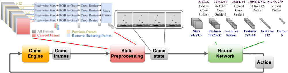
The input data given by the Atari Gym environment is an image with pixel size of 210x160 and 3 color channels. Following the pre-preprocessing procedure proposed by Mnih et al. [2013], the image is resized and stacked into 4 consecutive frames resulting in an image tensor of size 84x84x4. In order to speed up the policy evaluation step in Algorithm 1, every 4th frame is collected instead of collecting over each frame.
4 Evolution Strategy with Progressive Episode Lengths
In this section, we introduce Progressive Episode Lengths, discuss its components and show how we incorporate it into canonical ES.
4.1 Problems of Canonical ES
Although Chrabaszcz et al. [2018] showed that ES can perform quite well quantitatively, i.e., reaching a good score, the learned policies are quite poor from a qualitative perspective of humans. For example, in the game of Pong, a trained agent might score quite well, but fails to hit even easy balls reliably, an easy task for human players. The same observation applies to other Atari games as well in which the agent follows a good strategy to maximize its main scores, but fails to solve easy tasks and to play in a natural way. This leads to a brittle performance and high variance.
4.2 PEL: Progressive Episode Lengths
Inspired by the human strategy to first learn short and easy tasks, before learning the hard tasks, we propose to use progressive episode lengths (PEL), i.e., first train an agent to play short episodes and then based on the experience gained on these short episodes, train an agent on longer episodes.
The PEL approach is based on incremental learning, where an agent utilizes the capabilities obtained in limited games to an entire episodic run. The goal of this approach is to achieve more stable and faster optimization process by focusing on simpler and shorter tasks first. When integrating it with canonical ES, the latter is able to optimize by only playing a portion of a game, transferring the abilities obtained in a short game to a longer one. For example in the game of Pong, by solely learning to hit the ball, the algorithm could learn to play an entire game.
Another important advantage of the proposed PEL is that the ES approach can evaluate more policies by playing shorter games and thus, it can potentially make progress much faster. This applies in particular to tasks in RL, since the most timeconsuming step is often the evaluation of policies and not the ES-update of the policies. For the case of Atari games, these games typically last until the player loses all its in-game lives, which can take quite some time in certain games even if only a simple policy is applied. Therefore, limited episode lengths for evaluating more policies can speed up the optimization process substantially.
We formalized the idea of PEL in Algorithm 2. The input to PEL are two components: (i) the time scheduler T and (ii) the episode scheduler E (both discussed in the next subsections) and a maximal number of iterations (or another budget for running PEL). First we initialize the policy randomly (Line 1). In each iteration n, we update the maximal episode length using E (Line 3) and the time limit using T (Line 4) depending on n - 1 to run ES given an initial policy θn-1 (Line 5). The further improved policy θn returned by ES is used in the next iteration with potentially larger budgets.
4.3 Episode Scheduler
One of the main components of PEL is the episode scheduler to determine how many steps an episode should have at most. Partially following the idea of successive halving by Karnin et al. [2013], we propose a simple, yet effective episode scheduler that doubles the maximal episode length in each step, i.e., E(n) = 2n · E(0).
In preliminary experiments, we observed that in practice an important design decision is how to initialize the episode scheduler with E(0)-similar to the important minimal budget in successive halving and approaches build upon it [Li et al., 2017; Falkner et al., 2018]. For playing Atari games, we found that using the expected number of steps in playing random games is a good first estimate for E(0). However, on some games even more aggressive strategies can be beneficial
Algorithm 2: ES-based Progressive Episode Length
Input:
E - Episode Scheduler T - Time Scheduler N - Maximal number of iterations 1 Initialize a policy from normal distribution θ0 ∼N; 2 for n ∈ {1, . . . ,N} do 3 Set episode length according to E(n-1); 4 Set time limit according to T(n-1); /* Perform ES as in Algorithm 1 */ 5 θn ← ES(θn-1, T (n - 1), E(n - 1)); 6 end Output: θN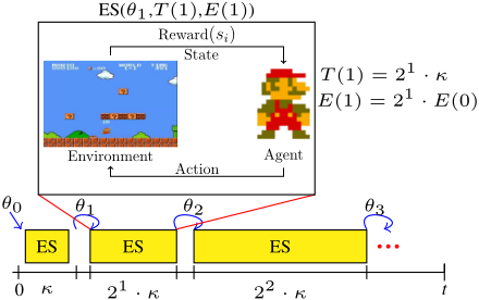
such that we initialize E(0) by the expected number of steps in playing random games divided by a constant; we used 2 in our experiments. 1 To approximate the expectation, we used Monte-Carlo roll-outs.
4.4 Time Scheduler
The second main component of PEL is the time scheduler T(n) defining how long to run ES given a limited episode length E(n). We propose two simple but yet effective schedulers. The first scheduler simply uses the time uniformly, i.e., T(n) is constant (in our experiments, we used 1 hour). The second schedule is again motivated by successive halving [Karnin et al., 2013] such that we double the time budget in each iteration, i.e., T(n) = 2n · κ for some user-defined κ (20min in our experiments). Using the second scheduler combined with our proposed episode scheduler, PEL will spend half of its overall optimization budget on the maximal episode length. Therefore, even if our heuristic assumption of learning on short games how to play long games should not hold, PEL will still focus on long games for most of its optimization budget.
4.5 An Example for PEL on Evolution Strategies
Figure 2 illustrates an instance of PEL where we double the episode length and the time frame simultaneously. To play a game for a total time budget t, runs of ES with different limited episodes are carried out. For each of these maximal episode lengths, the canonical ES is performed for a time limit defined by the time scheduler. For example in Figure 2, in the second iteration, n = 2, the ES algorithm starts its optimization loop from the policy θ1 which is passed from the first iteration. The ES evaluates episodes with at most E(1) actions, which is twice as much as in the previous iteration. Furthermore, the ES algorithm itself runs for at most T(1) (e.g., seconds or generations). The improved policy θ2 is then passed to the third run of ES.
1 We show all further empirical results in an online appendix.
5 Experiments
In this section, we will address the following research questions:
- Q1 How does PEL compare to the canonical ES by Chrabaszcz et al. [2018] for playing Atari games?
- Q2 How well do the proposed time schedulers perform?
- Q3 Is it possible to learn well-performing policies for long games by training only on short games?
5.1 Experimental Setup
To evaluate the performance of our proposed algorithm, we used a set of Atari games [Chrabaszcz et al., 2018] from OpenAI Gym [Brockman et al., 2016] and used the parallelization technique introduced by Salimans et al. [2017] that reduces the communication needed between workers. Each run used 400 CPUs on a high-performance cluster equipped with Intel Xeon E5-2630v4 processors and 128GB RAM.
We evaluated two time schedulers:
Tc →The time limit is set to a constant of 1 hour, Tc(n) = 1Td →The time limit is set to 20 minutes and doubled in each iteration, Td(n) = 20 · 2n .
Both versions use a doubling scheme to increase the maximal episode length. To compare PEL against canonical ES, we computed the relative improvement on each game and aggregated it by using a geometric mean. In our comparison, we used the same parametric setup for both PEL and canonical ES which is presented in Table 1. In order to estimate the initial episode length E(0) for PEL, we played each game multiple times using random actions and then divided by 2 the average number of actions until the episodes ended. To evaluate an approach, we ran five independent repetitions and evaluated the top found policy for 30 times. We report the mean evaluation scores of each of the five runs for both PEL (with Td and Tc) in comparison with canonical ES. 2
5.2 Q1: Comparison against Canonical ES
Table 2 shows our results for the two time schedulers Tc and Td and compare them to canonical ES. After 2 hours of training, the PEL approach with both schedulers outperformed the canonical ES in 5 and 6 games out of 9 and improved the scores by 49% and 80% on average, respectively. This shows the effectiveness of using the proposed PEL approach to improve the performance of canonical ES by optimizing different episode lengths, and utilizing the best-so-far policy of the previous iteration to improve further. After 10 hours, both schedulers are better than canonical ES in 7 out of 9 games, with an average improvement of 28% and 32% respectively. We conjecture that by running canonical ES for a longer time, the effect of PEL evaluating more policies decreases in comparison, such that the average improvement drops. On the other hand, PEL increases the episode lengths more often by running for 10 hours such that the PEL is more robust in this setting. (Please note that PEL with Tc increased the episode length only once within 2 hours).
2 We note that the code of Salimans et al. [2017] is not publicly available and Salimans et al. [2017] reported only a single run of their ES approach such that their performance estimate is potentially very noisy and not comparable with our results.
| Variable | Symbol | Value |
|---|---|---|
| Population size | λ | 800 |
| Parent population size | µ | 50 |
| Mutation step size | σ | 0.01 |
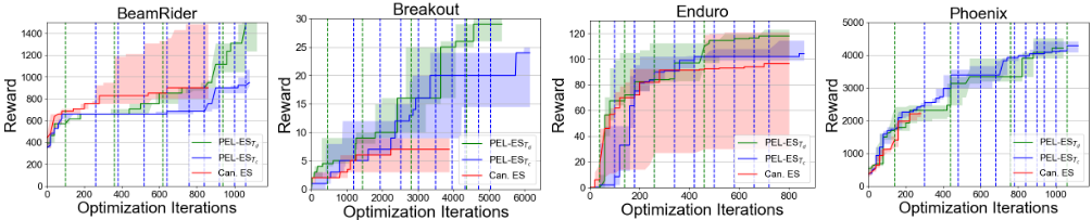
Figure 4 shows that PEL optimized for more iterations than canonical ES on most games, shown by the red line (canonical ES) which ends earlier than the green line (PEL with Td) and the blue line (PEL with Tc). On the game of Phoenix, it is obvious that this led to much better scores. However, on Enduro all approaches performed nearly the same amount of iterations; nevertheless, PEL achieved higher scores and had a much smaller variance across our repeated experiments (shown by a smaller shaded area).
Playing the game SpaceInvaders, PEL performed worse than canonical ES. In this specific game, the agent trained by PEL has never seen a major event in the game after optimizing for 2 hours: the arrival of the mothership which provides many points by shooting it. Therefore, PEL struggled to learn shooting the mothership reliably and obtained smaller scores on average.
5.3 Q2: Comparison of Time Schedulers
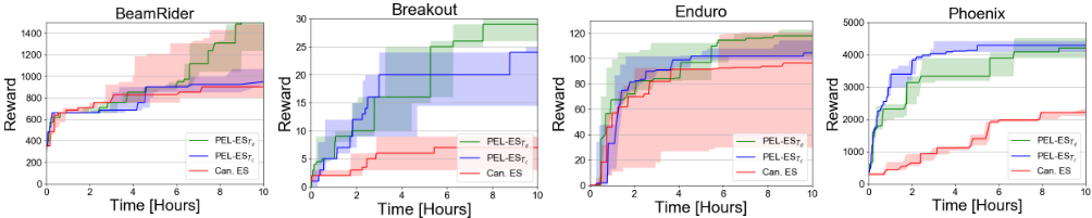
Comparing both schedulers, Td performed better in 6 out of 9 games both after 2 and 10 hours. The average improvement of Td after 2 hours is much higher than Tc's, but it is quite similar after 10 hours. To study the performance of both approaches over time in more detail, Figure 3 shows the performance of the best-so-far found policy evaluated on the full game lengths at each time point. Td performed particularly well after the first 5 hours and benefited from running longer games later on more than Tc. We draw a similar conclusion from studying the performance over the number of iterations (i.e., updates of the population), as shown in Figure 4.
5.4 Q3: Learning on Short Games
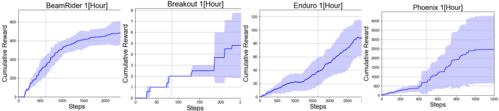
In order to verify whether an agent can learn a reasonable policy on short games, we studied the performance of PEL with Tc after 2 hours. At this point, PEL has not seen the full game, as shown in Figure 5 by the vertical lines. Nevertheless, PEL was able to find policies that played well on these short games (until the vertical line), but which are also able to perform well if we let them continue playing the games (after the vertical line). This verifies that the policies found by ES generalize to longer games and therefore, PEL is an efficient approach on these games.
6 Discussion and FutureWork
We introduced a new approach dubbed Progressive Episode Lengths (PEL) and integrated it with (canonical) ES. The main idea of PEL is to divide the time budget into differently limited time slots, and perform ES for each to firstly focus on solving simple tasks (e.g., shorter games). We then use the policies found on these short games to warm start ES to run on harder tasks (e.g., longer games) which leads to better results. We evaluated the performance of PEL on a set of Atari games from OpenAI Gym, and the results demonstrate that the proposed approach is able to provide better results compared to canonical ES, which always evaluated on full games.
The PEL approach has several assumptions: (i) We can find a well-performing policy on short games that generalizes well to longer games. We showed that this holds for many Atari games. For other tasks with sparse rewards or substantially delayed rewards, our approach has some limitations and will likely not perform well if the agent needs to play for a long time to get some rewards. Nevertheless, the PEL approach will not entirely fail in such tasks but it will lead to a slowdown such that the agent is still able to learn well. In the future, we will study whether this also holds for other RLtasks such as MuJoCo. (ii) We initialize our minimal episode length by playing random games. For games with a survival component, this often provides a reasonable starting point. However, preliminary results already indicate that for some Atari games a more aggressive strategy and for some others a less aggressive strategy will perform better. For RL-tasks with no natural episode lengths and for tasks where shorter episodes increase the difficulty, this heuristic will fail. Therefore, future work will include finding a more reliable heuristic to initialize episode lengths, and to start the evolution from different game fragments instead of playing the game from the beginning all the time.
Another direction for future work is to include a selfadapting scheduler such that the maximum number of allowed actions can be increased or decreased based on a potentially learned heuristic. Also, ES in its current form explores its environment by injecting random noise to its policy vector. Introducing a guided exploration by estimating the direction of a more rewarding space can improve the optimization process. Overall, we believe that integrating PEL into deep reinforcement learning algorithms is a promising direction and can lead to new advances in the state of the art.
Acknowledgments
Robert Bosch GmbH is acknowledged for financial support. The authors acknowledge support by the state of BadenW¨urrtemberg through bwHPC and the German Research Foundation (DFG) through grant no. INST 39/963-1 FUGG.
| Game | 2H | 10H | ||||
|---|---|---|---|---|---|---|
| Can. ES | PEL-ESTc | PEL-ESTd | Can. ES | PEL-ESTc | PEL-ESTd | |
| Alien | 1962 | 3673.4 | 3108.2 | 4063 | 5763.6 | 5509.6 |
| BankHeist | 41.6 | 214.2 | 229.8 | 192.4 | 341.8 | 269.4 |
| BeamRider | 743 | 718 | 734.8 | 1259 | 1107.6 | 1744.2 |
| Breakout | 16.4 | 10 | 44.8 | 64.6 | 110.4 | 120.2 |
| Enduro | 55.6 | 82.4 | 88 | 78.6 | 106 | 108.6 |
| Phoenix | 1011.6 | 3330.8 | 2872.6 | 2203.2 | 3821.6 | 3888.2 |
| Pong | 4.8 | 9.6 | 14.4 | 11 | 14.2 | 15.2 |
| Seaquest | 1263 | 1008.2 | 797.2 | 1914.2 | 2123.6 | 1755 |
| SpaceInvaders | 960.8 | 790 | 930 | 2030.6 | 1448 | 1610.6 |
| Average Improvement | 49% | 80% | 28% | 32% | ||
@inproceedings{ijcai2019p172,
  title     = {An Evolution Strategy with Progressive Episode Lengths for Playing Games},
  author    = {Fuks, Lior and Awad, Noor and Hutter, Frank and Lindauer, Marius},
  booktitle = {Proceedings of the Twenty-Eighth International Joint Conference on
               Artificial Intelligence, {IJCAI-19}},
  publisher = {International Joint Conferences on Artificial Intelligence Organization},
  editor    = {Sarit Kraus},
  pages     = {1234--1240},
  year      = {2019},
  month     = {8},
  note      = {Main track},
  doi       = {10.24963/ijcai.2019/172},
  url       = {https://doi.org/10.24963/ijcai.2019/172},
}
TY - CPAPER TI - An Evolution Strategy with Progressive Episode Lengths for Playing Games AU - Fuks, Lior AU - Awad, Noor AU - Hutter, Frank AU - Lindauer, Marius T2 - Proceedings of the Twenty-Eighth International Joint Conference on Artificial Intelligence, IJCAI-19 PB - International Joint Conferences on Artificial Intelligence Organization PY - 2019 SP - 1234 EP - 1240 DO - 10.24963/ijcai.2019/172 UR - https://doi.org/10.24963/ijcai.2019/172 ER -Copied
Machine-readable versions of this paper, for tools and AI agents:





