
Deanonymizing Social Networks Using Structural Information
Proceedings of the Twenty-Eighth International Joint Conference on Artificial Intelligence. Main track. Pages 1213-1219.
https://doi.org/10.24963/ijcai.2019/169
Keywords
- Machine Learning Applications: Networks
- Agent-based and Multi-agent Systems: Computational Social Choice
- Heuristic Search and Game Playing: Combinatorial Search and Optimisation
Abstract
We study the following fundamental graph problem that models the important task of deanonymizing social networks. We are given a graph representing an eponymous social network and another graph, representing an anonymous social network, which has been produced by the original one after removing some of its nodes and adding some noise on the links. Our objective is to correctly associate as many nodes of the anonymous network as possible to their corresponding node in the eponymous network. We present two algorithms that attack the problem by exploiting only the structure of the two graphs. The first one exploits bipartite matching computations and is relatively fast. The second one is a local search heuristic which can use the outcome of our first algorithm as an initial solution and further improve it. We have applied our algorithms on inputs that have been produced by well-known random models for the generation of social networks as well as on inputs that use real social networks. Our algorithms can tolerate noise at the level of up to 10%. Interestingly, our results provide further evidence to which graph generation models are most suitable for modeling social networks and distinguish them from unrealistic ones.
- [Arvind et al., 2012] Vikraman Arvind, Johannes Köbler, Sebastian Kuhnert, and Yadu Vasudev. Approximate graph isomorphism. In Proceedings of the 37th International Symposium on Mathematical Foundations of Computer Science (MFCS), volume 7464 of Lecture Notes in Com- puter Science, pages 100-111. Springer, 2012.
- [Babai et al., 1980] László Babai, Paul Erdös, and Stan- ley M. Selkow. Random graph isomorphism. SIAM Jour- nal on Computing, 9(3):628-635, 1980.
- [Babai et al., 1983] L. Babai, W. M. Kantor, and E. M. Luks. Computational complexity and the classification of finite simple groups. In Proceedings of the 24th Annual Sympo- sium on Foundations of Computer Science (FOCS), pages 162-171, 1983.
- [Babai, 2016] László Babai. Graph isomorphism in quasipolynomial time. In Proceedings of the 48th An- nual ACM SIGACT Symposium on Theory of Computing (STOC), pages 684-697, 2016.
- [Backstrom et al., 2007] Lars Backstrom, Cynthia Dwork, and Jon Kleinberg. Wherefore art thou r3579x?: anonymized social networks, hidden patterns, and struc- tural steganography. In Proceedings of the 16th inter- national conference on World Wide Web, pages 181-190, 2007.
- [Barabási and Albert, 1999] Albert-László Barabási and Réka Albert. Emergence of scaling in random networks. Science, 286:509-512, 1999.
- [Bollobás, 2001] Bella Bollobás. Random Graphs. Cam- bridge University Press, 2001.
- [Conte et al., 2004] Donatello Conte, Pasquale Foggia, Carlo Sansone, and Mario Vento. Thirty years of graph matching in pattern recognition. International Jour- nal of Pattern Recognition and Artificial Intelligence, 18(3):265-298, 2004.
- [Czajka and Pandurangan, 2008] Tomek Czajka and Gopal Pandurangan. Improved random graph isomorphism. Journal of Discrete Algorithms, 6(1):85-92, 2008.
- [Gilbert, 1959] E. N. Gilbert. Random graphs. The Annals of Mathematical Statistics, 30(4):1141-1144, 1959.
- [Grohe et al., 2018] Martin Grohe, Gaurav Rattan, and Ger- hard J. Woeginger. Graph similarity and approximate iso- morphism. In 43rd International Symposium on Mathe- matical Foundations of Computer Science (MFCS 2018), volume 117 of Leibniz International Proceedings in Infor- matics (LIPIcs), pages 20:1-20:16, 2018.
- [Hagberg et al., 2008] Aric A. Hagberg, Daniel A. Schult, and Pieter J. Swart. Exploring network structure, dynam- ics, and function using NetworkX. In Proceedings of the 7th Python in Science Conference (SciPy), pages 11-15, 2008.
- [Holme and Kim, 2002] Petter Holme and Beom Jun Kim. Growing scale-free networks with tunable clustering. Physical Review E, 65(2):026107:1-4, 2002.
- [Jiang et al., 2017] Honglu Jiang, Jiguo Yu, Chunqiang Hu, Cheng Zhang, and Xiuzhen Cheng. SA framework based de-anonymization of social networks. In Proceedings of the 2017 International Conference on Identification, In- formation and Knowledge in the Internet of Things (IIKI), pages 358-363, 2017.
- [Kazemi et al., 2015] Ehsan Kazemi, S. Hamed Hassani, and Matthias Grossglauser. Growing a graph matching from a handful of seeds. Proceeding of the VLDB Endowment, 8(10):1010-1021, 2015.
- [Leskovec and Krevl, 2014] Jure Leskovec and Andrej Krevl. SNAP Datasets: Stanford large network dataset collection. http://snap.stanford.edu/data, June 2014. Link
- [McKay and Piperno, 2014] Brendan D. McKay and Adolfo Piperno. Practical graph isomorphism, II. Journal of Sym- bolic Computation, 60:94 -112, 2014.
- [Narayanan and Shmatikov, 2009] Arvind Narayanan and Vitaly Shmatikov. De-anonymizing social networks. In IEEE Symposium on Security and Privacy, pages 173- 187. IEEE Computer Society, 2009.
- [Pedarsani and Grossglauser, 2011] Pedram Pedarsani and Matthias Grossglauser. On the privacy of anonymized net- works. In Proceedings of the 17th ACM SIGKDD Inter- national Conference on Knowledge Discovery and Data Mining (KDD), pages 1235-1243, 2011.
- [Qian et al., 2017] Jianwei Qian, Xiang-Yang Li, Yu Wang, Shaojie Tang, Taeho Jung, and Yang Fan. Social network de-anonymization: more adversarial knowledge, more users re-identified? CoRR, abs/1710.10998, 2017.
- [Rossi and Ahmed, 2015] Ryan A. Rossi and Nesreen K. Ahmed. The network data repository with interactive graph analytics and visualization. In Proceedings of the 29th AAAI Conference on Artificial Intelligence (AAAI), 2015.
- [Watts and Strogatz, 1998] Duncan J. Watts and Steven H. Strogatz. Collective dynamics of small-world networks. Nature, 393:440-442, 1998.
References were extracted automatically from the PDF and may contain errors.
Full text extracted automatically from the PDF; figures, tables and equations may differ. The PDF is the version of record.
1 Introduction
Privacy is undoubtedly an invaluable resource in today's communication networks, and much of the activities of leading institutions on the Internet focus on protecting the privacy of users. However, this may facilitate illegal activities which have to be uncovered. In this paper, we study the problem of deanonymizing an anonymous social network. Our aim is to use only information about the network structure and deanonymize it by trying to match its structure to that of a broader social network with known node identities.
More concretely, we study the following problem. We are given an eponymous social network G and another anonymous social network H. H is a noisy subgraph of G in the following sense. All nodes of H also appear in G (but there may be nodes in G which do not appear in H), but the information about the identities of the nodes of H and their correspondence to nodes of G is not available. The set of edges of H is an "approximation" of the edge set of G; for every pair of nodes that exists in both G and H, the probability that their edge relationship is different in the two graphs is low (but typically non-zero). Ideally, we would like to compute the correspondence of the nodes of H to the nodes of G that correctly recovers the identity of the nodes of H. We would like to do so using structural information, i.e., using only the graph representation of the two social networks.
We assume that no mechanism to verify the identity of a node of H is available. Still, we would like to compute a node correspondence that is as close to the underlying true one as possible. This quest makes sense only if H is a noisy estimate of G (with low noise levels so that the two networks are not very different). When designing deanonymization algorithms, we will pessimistically assume that no specific noise parameters are available and we would like to identify the nodes of H by trying to match the two graphs in the best way. Informally, the intermediate problemwe will solve in order to come up with a good deanonymization is to compute a node correspondence that recovers the maximum number of edge relationships between node pairs.
In particular, we present two algorithms. Our first one is inspired by an idea that originates from a paper by Babai et al. [1980] on the graph isomorphism problem of random graphs and exploits bipartite matchings. The second one exploits local search in order to find the seemingly best possible match between the two graphs by continuously making local improvements on the node correspondence. Formal analysis is used to bound the running time of the second algorithm. Experimental results show that by combining the two algorithms, we can tolerate noise at the level of up to 10% and deanonymize correctly large fractions of the network nodes.
1.1 RelatedWork
Deanonymization of social networks became popular ten years ago with the work of Narayanan and Shmatikov [2009]. In their paper, they relate privacy to anonymity and show that the usual practice of network operators to share sensitive information about users with advertisers, application developers, and data-mining researchers after anonymizing data (e.g., removing names) can severely violate privacy. Privacy violation has been the focus of several papers. Notable among them is the paper by Backstrom et al. [2007], who assume that an adversary is able to modify the network before its release. Such approaches use new "sybil" nodes and usually require the in advance identification of a small number of seed nodes.
Our approach here is fundamentally different. We assume the existence of a known eponymous social network and an anonymous social network, where criminal or illegal activity takes place. Information about the structure of both networks is available, and the objective is to match the two structures in the best possible way so that the node identities of as many nodes in the anonymous network are revealed. No other information about the networks (such as node attributes, some initial set of already identified nodes, etc.) is available. Ideally, one would be interested in a graph isomorphism solution. Graph isomorphism received much attention recently through the celebrated result of Babai [2016], who improved on previous work from the '80s [Babai et al., 1983]. In the decision version of the graph isomorphism problem, we are given two graphs, and we would like to decide whether they are isomorphic or not. In its search version, we would also like to recover the node correspondence between the two graphs in case they are isomorphic. The problem has been proved to be challenging only in theory; in practice, it is well-known to be efficiently solvable; e.g., see [McKay and Piperno, 2014].
Unfortunately, the eponymous and the anonymous social networks are never identical. Hence, an optimization version of graph isomorphism has to be solved. Several objectives have been considered in the related literature, such as maximizing the number of edge matches [Arvind et al., 2012] or minimizing the Frobenius distance [Grohe et al., 2018]. Pedarsani and Grossglauser [2011] and Kazemi et al. [2015] consider settings with additional available information, such as seeds of identified nodes. These papers follow a theoretical approach. Variations of these settings are considered by Qian et al. [2017] and Jiang et al. [2017]. A survey on more practical aspects of "graph matching" from the pattern recognition literature can be found in [Conte et al., 2004]. However, none of these conceptually related papers considers the particular setting and performance objective of the current paper.
2 Preliminaries
We begin with preliminary definitions. For a graph G, we denote by V (G) and E(G) the sets of nodes and edges, respectively. Consider two graphs G and H with |V (G)| ≥ |V (H)| and define a function F : V (G) → V (H) ∪ {0} which associates each node of V (G) either to a distinct node of V (H) or to the dummy node 0. For every node v of V (H), there is exactly one node u of V (G) with F(u) = v; hence, |V (G)| - |V (H)| nodes of V (G) are mapped to 0. We refer to function F using the term pseudobijection.
We will formally define the deanonymization (or reidentification) problem in social networks. The input consists of two graphs G and H. Graph G has n nodes which are identified as the positive integers in the set [n]. Graph H has been obtained from G using three steps:
- First, a permutation is applied to the nodes of G.
- Second, some of the nodes of G are removed.
- Third, some of the edges of G are replaced by new edges.
Using the notation introduced in the previous paragraph, this process essentially defines a pseudobijection F ∗ of the nodes of G to the nodes of H and the dummy node 0. The objective of the reidentification problem is, given the two graphs G and H, to recover the pseudobijection F ∗ as accurately as possible. The performance of a deanonymization algorithm that returns a pseudobijection F is measured as
where II {X} is equal to 1 if the condition X is true and is equal to 0 otherwise.
We aim to design deanonymization algorithms of high performance. We present two algorithms which are presented in the next two sections. The first algorithm exploits and extends an idea that originates from solutions for the graph isomorphism problem in random graphs. In particular, let us consider as input graph G a graph following the Gn,p model, which produces graphs with n nodes in which each possible edge between pairs of nodes exists with probability p (independently from other edges). Further, assume that the graph H is isomorphic to G, i.e., it has been obtained by just applying step 1 in the process described above. As Babai et al. [1980] observed, the sorted sequence of degrees in the neighborhood of a node of an Gn,1/2 Erd¨os-Renyi random graph is unique with high probability. This property carries over for different values of p; see the results by Bollobas [2001, Theorem 3.17, page 74] and Czajka and Pandurangan [2008]. Hence, the neighbor degree sequence can be used as a node identifier and the correct association of the nodes of graphs G and H can be found efficiently, with high probability.
In our more general reidentification problem in which the graph G is not necessarily an Erd¨os-Renyi graph and steps 2 and 3 will have typically be applied to graph G, neighbor degree sequence is not a unique node identifier anymore. Still, the main idea of our first algorithm is to compute a pseudobijection between nodes of graphs G and H by computing the best match of nodes between G and H based on the neighbor degree sequence difference.
3 Deanonymization via aMatching Computation
Our first algorithm, called Neighbor Degree Sequence Difference (NDSD for short), computes a pseudobijection from V (G) to V (H) as follows. It first adds dummy isolated nodes to graph H (these will be used for mapping nodes of V (G) to 0). Then, it computes the quantity diff(u, v) denoting the difference in the local structure between a node u in graph G and either an original or a dummy node v in graph H. Now, diff(u, v) is computed as follows. For a node u of G (respectively, either an original or a dummy node v of H), let degu (resp., degv ) be the (|V (G)| - 1)-entry vector containing the degrees of the neighbors of node u in G (resp., of node v in H) sorted in non-increasing order, with zeros in the missing entries (if any). Then,
We will refer to vector degu as the degree sequence of node u. By definition, a dummy node has a degree sequence consisting of zeros.
Then, our NDSD algorithm computes a minimum-weight perfect matching in an edge-weighted complete bipartite graph (here, we have used a standard implementation of the Hungarian method which runs in O(n4 ) time) which has a left node for each node u of graph G and a right node for each original node of H and for each dummy node that is added on it. The weight of the edge corresponding to the pair (u, v) is equal to diff(u, v). The perfect matching defines a pseudobijection F : V (G) → V (H) ∪ {0} in the obvious way, i.e., F(u) = 0 or F(u) = v if the perfect matching contains an edge between node u and a dummy or non-dummy node v, respectively. Essentially, the perfect matching returned by the algorithm minimizes the quantity
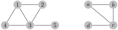
Let us consider the two graphs of Figure 1 as an example. As graph G has one more node than H, we add the dummy node e to H before computing the degree sequences. The degree sequences of all nodes are:
| 1 : | 4 | 2 | 2 | 0 | a | : | 3 | 2 | 0 0 | |
| 2 : | 4 | 3 | 0 | 0 | b | : | 3 | 2 | 0 | 0 |
| 3 : | 3 | 2 | 2 | 1 | c | : | 2 | 2 | 1 0 | |
| 4 : | 4 | 3 | 0 | 0 | d | : | 3 | 0 | 0 | 0 |
| 5 : | 4 | 0 | 0 | 0 | e | : | 0 | 0 | 0 | 0 |
Applying (1), we get the edge weights
| a | b | c | d | e |
|---|---|---|---|---|
| 1 3 | 3 | 3 | 5 | 8 |
| 2 2 | 2 | 4 | 4 | 7 |
| 3 3 | 3 | 3 | 5 | 8 |
| 4 2 | 2 | 4 | 4 | 7 |
| 5 3 | 3 | 5 | 1 | 4 |
The circles indicate a minimum-weight perfect matching. The corresponding pseudobijection is then defined as F (1) = a, F(2) = 0, F(3) = c, F(4) = b, and F(5) = d.
4 A Local Search Algorithm
In order to describe our local search algorithm, we will need some additional notation. For two nodes u and v of G, we define the binary quantity adjF (u, v) to be equal to 0 if some (or both) of the nodes are mapped to 0 under F and as
otherwise. Intuitively, the binary quantity adjF (u, v) indicates whether the pseudobijection F preserves the adjacency information between nodes u and v in both G and H.
For a pseudobijection F and a node u ∈ V (G), define the quality of F for node u to be 0 if F(u) = 0 and as
otherwise. So, clearly, the quality of F for node u is nonnegative and at most n - 1.
Our local search algorithm (Algorithm 1) starts with a pseudobijection F, which repeatedly tries to improve. In each attempt for improvement (i.e., in each execution of the for loop in lines 6-16), the algorithm examines every pair of nodes u1 and u2 and considers swapping their images under F; this yields a neighboring pseudobijection F ′ of F. If the total quality of nodes u1 and u2 strictly increases in F ′ (compared to F, i.e., if qualF ′(u1) + qualF ′(u2) > qualF (u1)+qualF (u2)), the algorithm keeps the new pseudobijection. It terminates when, after examining all pairs of nodes of V (G), no improved pseudobijection is found. On termination, the updated pseudobijection is returned.
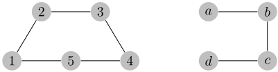
Assume that we run the local search algorithm with input the graphs G and H of Figure 2 and let F be the initial pseudobijection defined as F(1) = a, F(2) = c, F(3) = b, F(4) = 0, F(5) = d. It can be easily seen that this is a pseudobijection that could have been returned as the solution of algorithm NDSD. Now, consider the pair of nodes 1 and 4 in graph G; their qualities under F are both 0. By swapping the images of nodes 1 and 4 (let this be pseudobijection F ′ ), we get qualities 0 (for 1) and 2 (for 4, since adjF ′(4, 2) = adjF ′(4, 3) = 1). Hence, this neighboring pseudobijection becomes the current pseudobijection F. Then, observe that the qualities of the nodes 1 and 5 are 0 and 1 (since adjF (5, 3) = 1), respectively. By swapping the images of nodes 1 and 5 (let this be pseudobijection F ′ now), we get improved qualities 3 (for 1) and 0 (for 5). After this one, no other improvement is possible and the final pseudobijection is F(1) = d, F(2) = c, F(3) = b, F(4) = a, and F (5) = e.
The worst-case performance of our algorithm is given by the next statement. We remark that the number of iterations is essentially the number of executions of the while loop. The actual running time is O(n5 ) as we have to take into account the execution of the for loop and the recomputation of qualities in line 8.
Theorem 1. On input two graphs G = (V (G),E(G)) and H = (V (H), E(H)) with |V (H)| ≤ |V (G)| = n, the local search algorithm terminates after O(n2 ) iterations.
Proof. We will show that the function
Algorithm 1 The local search algorithm
Input: graphs G and H with |V (G)| ≥ |V (H)| and initial pseudobijection F : V (G) → V (H) ∪ {0} Output: updated pseudobijection F : V (G) → V (H)∪{0} 1: compute quality qualF (u), ∀u ∈ G 2: change ← 1 3: while change do 4: change ← 0 5: F ′ ←F 6: for all u1, u2 ∈ G, with u1 ̸= u2 do 7: F ′ (u1) ← F (u2); F ′ (u2) ← F (u1) 8: compute qualities qualF ′ (u1) and qualF ′ (u2) 9: if qualF ′(u1) + qualF ′(u2) > qualF (u1) + qualF (u2) then 10: change ← 1 11: F (u1) ← F ′ (u1); F (u2) ← F ′ (u2) 12: update quality qualF (u), ∀u ∈ G 13: else 14: F ′ (u1) ← F (u1); F ′ (u2) ← F (u2) 15: end if 16: end for 17: end while 18: return Fdefined over all possible pseudobijections of V (G) to V (H) is a potential function for the local search algorithm. In particular, we will show that in every step in which the algorithm performs an improvement step and decides to discard the current pseudobijection F and replace it with a pseudobijection F ′ in which F(u) and F(v) are swapped (i.e., F ′ (u) = F(v) and F ′ (v) = F(u)) for some pair of nodes u, v ∈ V (G), the difference Φ(F ′ )-Φ(F) has value at least 2. As Φ is always non-negative and can never get a value higher than n(n - 1), an upper bound of n(n-1)/2 on the number of iterations for the local search algorithmwill follow.
By the definition of Φ, we have
Using this equality, the definition of qualF , and observing that F and F ′ differ only in the mapping of nodes u1 and u2, we have that
The second equality follows since the mappings of u1 and u2 are swapped in F and F ′ and, hence, adjF (u1, u2) =
adjF ′(u1, u2). By the definition of the algorithm, since it considers the new pseudobijection F ′ instead of the current one F, we have that the rightmost parenthesis has value at least 1 and the potentials differ by at least 2, as desired.
Observe that, when graphs G and H are isomorphic, there is a pseudobijection F (the isomorphism) which is an optimal solution to both algorithm NDSD and the local search algorithm. This is due to the fact that F yields diff(u, F (u)) = 0 for each u ∈ V (G) and, consequently, the perfect matching that connects every node u of G to node F(u) in H has zero weight. Furthermore, assuming that |V (G)| = |V (H)| = n, we have that qualF (u) = n - 1 (since adj(u, v) = 1 for every v ∈ V (G) \ {u}) and, hence, the potential Φ(F) has the highest possible value of n(n - 1).
On the other hand, the objectives used by the algorithms seem different, and it should be definitely expected that there are instances with different input graphs in which any pseudobijection (globally) optimizing the potential Φ has suboptimal ∆ and vice-versa. So, we obtain our best results by combining the two algorithms. Algorithm NDSD runs first and computes a pseudobijection that is used as the initial pseudobijection of the local search algorithm. This, of course, means that the potential of the pseudobijection obtained by the local search algorithm is at least as large as the initial one but this does not exclude the existence of a pseudobijection with a significantly higher potential that is missed because local search is trapped in a local maximum.
5 Experimental Results
We have implemented in C both the NDSD and the local search algorithm and have used them in all our experiments. 1 NDSD runs either on isolation on input instances or is used to compute the initial solution, which is then further improved by the local search algorithm. This combination has been selected among other variations with inferior performance (e.g., random selection of the initial solution, simpler local search heuristics, etc.).
As input to our algorithms, we have used graphs that represent snapshots of (parts of) real social networks as well as random graphs produced by well-known models for graph generation. The real-world instances include the ego-facebook graph from the SNAP collection of social networks [Leskovec and Krevl, 2014] as well as sixteen facebook graphs from the Network Repository [Rossi and Ahmed, 2015]. Among the several datasets in SNAP, ego-facebook is the only undirected graph of moderate size (4K nodes and 88K edges). The instances from the Network Repository have between 1.4K and 3.5K nodes and between 33K and 155K edges (see detailed data in Table 1; data are from [Rossi and Ahmed, 2015] and [Leskovec and Krevl, 2014]).
In our experiments we have used instances of random graphs, generated with four different models (using their implementation in NetworkX [Hagberg et al., 2008]), namely the Erd¨os-R´enyi Gn,p model [Gilbert, 1959], the WattsStrogatz for generating small-world graphs [Watts and Strogatz, 1998], the Barab´asi-Albert preferential attachment model [Barab´asi and Albert, 1999], and the algorithm by Holme and Kim [2002]. The last two models are well-known (in addition to the Gn,p and the Watts-Strogatz models) for building graphs with power-law degree distribution. As such, they are considered more realistic ones in modeling social networks. All the above models have been used to produce graphs with 1K nodes and approximately 35K edges. These graphs are slightly smaller than but of comparable density to the real-world instances we have used.
1 Our computational results (including what we report here as well as additional ones that we omit due to lack of space) have been obtained using a desktop PC with an Intel i7-4790/3.6GHz processor with 8GB of RAM, running a Slackware64 operating system. The total computation time of all experiments has exceeded 200 hours.
| network name | #nodes | #edges | maximum degree |
|---|---|---|---|
| Amherst41 | 2235 | 90954 | 467 |
| Bowdoin47 | 2252 | 84387 | 670 |
| Colgate88 | 3482 | 155043 | 773 |
| Hamilton46 | 2314 | 96394 | 602 |
| Haverford76 | 1446 | 59589 | 375 |
| Middlebury45 | 3075 | 124610 | 473 |
| Oberlin44 | 2920 | 89912 | 478 |
| Pepperdine86 | 3445 | 152007 | 674 |
| Simmons81 | 1518 | 32988 | 300 |
| Smith60 | 2970 | 97133 | 349 |
| Swarthmore42 | 1659 | 61050 | 577 |
| Trinity100 | 2613 | 111996 | 404 |
| USFCS72 | 2682 | 65252 | 405 |
| Vassar85 | 3068 | 119161 | 482 |
| Wellesley22 | 2970 | 94899 | 746 |
| Williams40 | 2790 | 112986 | 610 |
| Ego-facebook | 4039 | 88234 | 1045 |
The above graphs (either the real-world ones or the ones generated by the four generators) form the eponymous social network. Following the terminology in Section 2, we refer to them as graph G. Then, graph H is produced as follows. First, some nodes are removed from G, and some edges are replaced by random ones; this gives graph H which represents the anonymous social network. Essentially, graph H is a noisy estimate of graph G, in which any identification of the nodes has been removed. This is implemented by changing the node IDs by taking a random permutation of them.
In particular, we build H from G using two parameters, δ and ϵ. The parameter δ indicates the fraction of nodes that are removed from graph G together with their incident edges. Next, we remove an ϵ fraction of the edges that survived and replace each of them by a random (new) edge in the graph. In our experiments with real-world data from the Network Repository, we have used different values between 0 and 20% for δ and between 0 and 10% for ϵ. In our experiments with randomly generated social networks or with ego-facebook, we have used a smaller range of values for δ, between 0 and 10% (and, again, values between 0 and 10% for ϵ).
Now, the particular way graph H is obtained by G implies a hidden true pseudo-bijection, according to which each node of H is mapped to a node of G. In our experiments, we compare the pseudo-bijections computed by the algorithms to this hidden true one and require from an optimal pseudobijection to coincide with the latter. In all experiments, we measure the correctly recovered identifications of the nodes of graph H and express this quantity as a fraction. So, a performance of 90% means that 90% of the nodes of H are mapped to their correct node in graph G. As we will see, the algorithms can achieve performance approaching 100% and recover the pseudo-bijection exactly or almost exactly for reasonable noise levels.
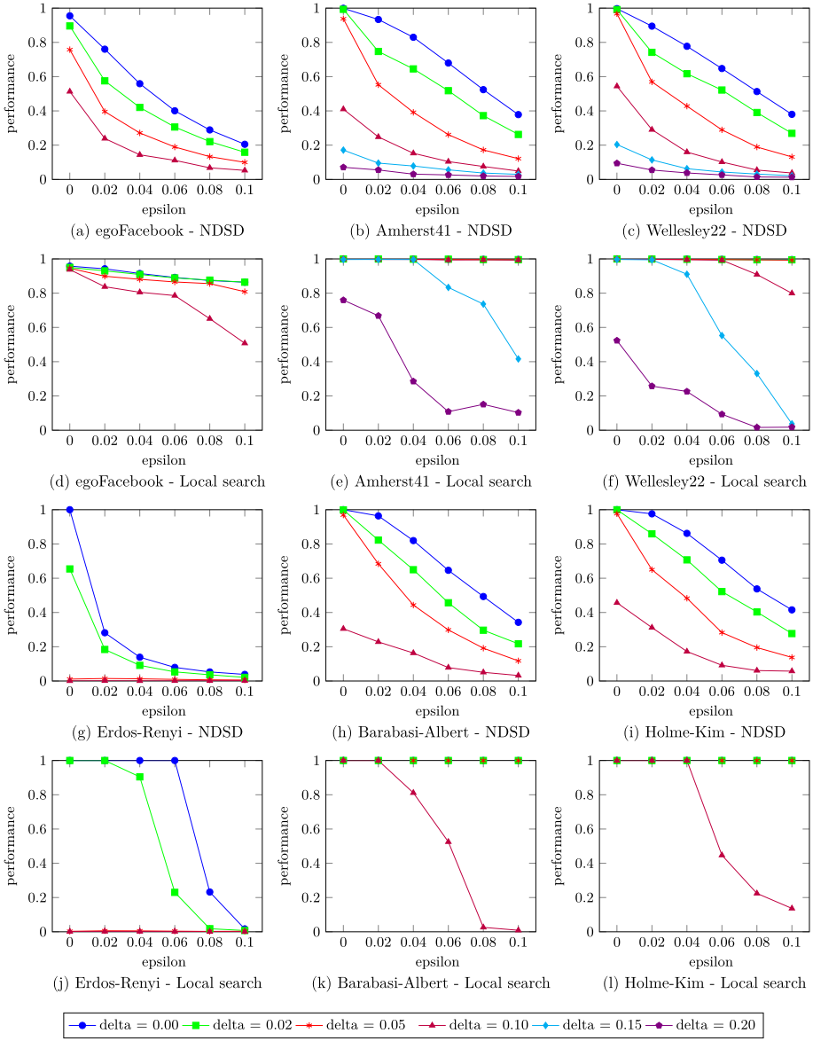
Our results from the execution of NDSD and the local search algorithm are depicted in Figure 3. In the sixteen instances from the Network Repository, NDSD recovers the optimal (or almost optimal) pseudo-bijection when there is no noise in the edges and the noise level for nodes is at most 5%. Results are suboptimal for higher noise levels, but performance drops gracefully (see Figures 3b and 3c). The local search algorithm performs even better (see Figures 3e and 3f). Recall that this algorithm uses the NDSD solution as an initial point, which is then further improved. Our experiments indicate that for noise levels of at most 10% for nodes and edges, local search returns optimal solutions for most real networks, except for Oberlin44, Pepperdine86, Smith60, and Wellesley22, which have suboptimal performance for edge and node noise of 10%. Figure 3f is representative of the performance of our local search algorithm on these networks while Figure 3e is representative of the remaining real social network from the Network Repository. For node noise of 15% or 20%, the performance of local search drops, but with a similar pattern across all real networks from the Network Repository. The results for ego-facebook are very similar; there seems to be a small decrease in performance that was not observed in the other real networks for small noise values (see Figures 3a and 3d).
The performance of the algorithms on random graphs follows different patterns that depend on the generation model. The Watt-Strogatz and Erdos-Renyi inputs seem to be on one extreme. Besides the case of zero noise levels, the NDSD algorithm has poor performance on Watts-Strogatz graphs. Not surprisingly, the local search has poor performance too. The behaviour of the algorithms on Erdos-Renyi graphs is more interesting. NDSD still has poor performance in the presence of noise. Somewhat surprisingly, the local search algorithm is able to considerably improve the initial solution at least for node noise up to 2% and edge noise of at most 4%. The Barabasi-Albert and Holme-Kim inputs are on the other extreme in the sense that the results are in sync with those in the real networks, both for the NDSD and the local search algorithm. These results are depicted in Figures 3g-3l.
To conclude, the message from our results is two-fold. First, the combination of NDSD and the local search algorithm yields very good reidentification in the presence of reasonable levels of noise. Secondly, the random graph models of Barabasi-Albert and Holme-Kim seem to be closer to all real networks we considered, at least as far as the behaviour of our algorithms is concerned. Our results for Watt-Strogatz and Erdos-Renyi inputs support the firm belief that these models are unsuitable for modeling real social networks.
@inproceedings{ijcai2019p169,
  title     = {Deanonymizing Social Networks Using Structural Information},
  author    = {Caragiannis, Ioannis and Tsitsoka, Evanthia},
  booktitle = {Proceedings of the Twenty-Eighth International Joint Conference on
               Artificial Intelligence, {IJCAI-19}},
  publisher = {International Joint Conferences on Artificial Intelligence Organization},
  editor    = {Sarit Kraus},
  pages     = {1213--1219},
  year      = {2019},
  month     = {8},
  note      = {Main track},
  doi       = {10.24963/ijcai.2019/169},
  url       = {https://doi.org/10.24963/ijcai.2019/169},
}
TY - CPAPER TI - Deanonymizing Social Networks Using Structural Information AU - Caragiannis, Ioannis AU - Tsitsoka, Evanthia T2 - Proceedings of the Twenty-Eighth International Joint Conference on Artificial Intelligence, IJCAI-19 PB - International Joint Conferences on Artificial Intelligence Organization PY - 2019 SP - 1213 EP - 1219 DO - 10.24963/ijcai.2019/169 UR - https://doi.org/10.24963/ijcai.2019/169 ER -Copied
Machine-readable versions of this paper, for tools and AI agents:





