
Watching a Small Portion could be as Good as Watching All: Towards Efficient Video Classification
Proceedings of the Twenty-Seventh International Joint Conference on Artificial Intelligence. Main track. Pages 705-711.
https://doi.org/10.24963/ijcai.2018/98
Keywords
- Machine Learning Applications: Applications of Reinforcement Learning
- Computer Vision: Video: Events, Activities and Surveillance
Abstract
We aim to significantly reduce the computational cost for classification of temporally untrimmed videos while retaining similar accuracy. Existing video classification methods sample frames with a predefined frequency over entire video. Differently, we propose an end-to-end deep reinforcement approach which enables an agent to classify videos by watching a very small portion of frames like what we do. We make two main contributions. First, information is not equally distributed in video frames along time. An agent needs to watch more carefully when a clip is informative and skip the frames if they are redundant or irrelevant. The proposed approach enables the agent to adapt sampling rate to video content and skip most of the frames without the loss of information. Second, in order to have a confident decision, the number of frames that should be watched by an agent varies greatly from one video to another. We incorporate an adaptive stop network to measure confidence score and generate timely trigger to stop the agent watching videos, which improves efficiency without loss of accuracy. Our approach reduces the computational cost significantly for the large-scale YouTube-8M dataset, while the accuracy remains the same.
- [Abu-El-Haija et al., 2016] Sami Abu-El-Haija, Nisarg Kothari, Joonseok Lee, Paul Natsev, George Toderici, Balakrishnan Varadarajan, and Sudheendra Vijaya- narasimhan. Youtube-8m: A large-scale video classifica- tion benchmark. CoRR, abs/1609.08675, 2016.
- [Bhatnagar et al., 2017] Bharat Lal Bhatnagar, Suriya Singh, Chetan Arora, and C. V. Jawahar. Unsupervised learning of deep feature representation for clustering egocentric ac- tions. In IJCAI, 2017. IJCAI
- [Chang et al., 2016] Xiaojun Chang, Yi Yang, Guodong Long, Chengqi Zhang, and Alexander G. Hauptmann. Dy- namic concept composition for zero-example event detec- tion. In AAAI, 2016.
- [Fan et al., 2017] Hehe Fan, Xiaojun Chang, De Cheng, Yi Yang, Dong Xu, and Alexander G. Hauptmann. Com- plex event detection by identifying reliable shots from untrimmed videos. In ICCV, 2017.
- [He et al., 2016] Kaiming He, Xiangyu Zhang, Shaoqing Ren, and Jian Sun. Deep residual learning for image recog- nition. In CVPR, 2016.
- [Hochreiter and Schmidhuber, 1997] Sepp Hochreiter and Jürgen Schmidhuber. Long short-term memory. Neural Computation, 9(8):1735-1780, 1997.
- [Howard et al., 2017] Andrew G Howard, Menglong Zhu, Bo Chen, Dmitry Kalenichenko, Weijun Wang, Tobias Weyand, Marco Andreetto, and Hartwig Adam. Mo- bilenets: Efficient convolutional neural networks for mo- bile vision applications. arXiv preprint arXiv:1704.04861, 2017.
- [Jouppi et al., 2017] Norman P Jouppi, Cliff Young, Nishant Patil, David Patterson, Gaurav Agrawal, Raminder Bajwa, Sarah Bates, Suresh Bhatia, Nan Boden, Al Borchers, et al. In-datacenter performance analysis of a tensor processing unit. arXiv preprint arXiv:1704.04760, 2017.
- [Karpathy et al., 2014] Andrej Karpathy, George Toderici, Sanketh Shetty, Thomas Leung, Rahul Sukthankar, and Li Fei-Fei. Large-scale video classification with convo- lutional neural networks. In CVPR, 2014.
- [Krizhevsky et al., 2012] Alex Krizhevsky, Ilya Sutskever, and Geoffrey E. Hinton. Imagenet classification with deep convolutional neural networks. In NIPS, 2012.
- [Mnih et al., 2014] Volodymyr Mnih, Nicolas Heess, Alex Graves, and Koray Kavukcuoglu. Recurrent models of vi- sual attention. In NIPS, 2014.
- [Mnih et al., 2016] Volodymyr Mnih, Adrià Puigdomènech Badia, Mehdi Mirza, Alex Graves, Timothy P. Lillicrap, Tim Harley, David Silver, and Koray Kavukcuoglu. Asyn- chronous methods for deep reinforcement learning. In ICML, 2016.
- [Ng et al., 2015] Joe Yue-Hei Ng, Matthew Hausknecht, Sudheendra Vijayanarasimhan, Oriol Vinyals, Rajat Monga, and George Toderici. Beyond short snippets: Deep networks for video classification. In CVPR, 2015.
- [Pan et al., 2016] Pingbo Pan, Zhongwen Xu, Yi Yang, Fei Wu, and Yueting Zhuang. Hierarchical recurrent neural encoder for video representation with application to cap- tioning. In CVPR, 2016.
- [Simonyan and Zisserman, 2014] Karen Simonyan and An- drew Zisserman. Two-stream convolutional networks for action recognition in videos. In NIPS, 2014.
- [Simonyan and Zisserman, 2015] Karen Simonyan and An- drew Zisserman. Very deep convolutional networks for large-scale image recognition. In ICLR, 2015.
- [Szegedy et al., 2016] Christian Szegedy, Vincent Van- houcke, Sergey Ioffe, Jonathon Shlens, and Zbigniew Wojna. Rethinking the inception architecture for computer vision. In CVPR, 2016.
- [Tran et al., 2015] Du Tran, Lubomir Bourdev, Rob Fergus, Lorenzo Torresani, and Manohar Paluri. Learning spa- tiotemporal features with 3d convolutional networks. In ICCV, 2015.
- [Tran et al., 2017] Du Tran, Jamie Ray, Zheng Shou, Shih- Fu Chang, and Manohar Paluri. Convnet architecture search for spatiotemporal feature learning. arXiv preprint arXiv:1708.05038, 2017.
- [Venugopalan et al., 2015] Subhashini Venugopalan, Mar- cus Rohrbach, Jeff Donahue, Raymond Mooney, Trevor Darrell, and Kate Saenko. Sequence to sequence -video to text. In ICCV, 2015.
- [Wang and Schmid, 2013] Heng Wang and Cordelia Schmid. Action recognition with improved trajectories. In ICCV, 2013.
- [Wang et al., 2011] Heng Wang, Alexander Kläser, Cordelia Schmid, and Cheng-Lin Liu. Action recognition by dense trajectories. In CVPR, 2011.
- [Wang et al., 2016] Limin Wang, Yuanjun Xiong, Zhe Wang, Yu Qiao, Dahua Lin, Xiaoou Tang, and Luc Van Gool. Temporal segment networks: Towards good practices for deep action recognition. In ECCV, 2016.
- [Williams, 1992] Ronald J. Williams. Simple statistical gradient-following algorithms for connectionist reinforce- ment learning. Machine Learning, 8:229-256, 1992.
- [Xu et al., 2015] Zhongwen Xu, Yi Yang, and Alexander G. Hauptmann. A discriminative CNN video representation for event detection. In CVPR, 2015.
- [Yeung et al., 2016] Serena Yeung, Olga Russakovsky, Greg Mori, and Li Fei-Fei. End-to-end learning of action detec- tion from frame glimpses in videos. In CVPR, 2016.
- [Yue-Hei Ng et al., 2015] Joe Yue-Hei Ng, Matthew Hausknecht, Sudheendra Vijayanarasimhan, Oriol Vinyals, Rajat Monga, and George Toderici. Beyond short snippets: Deep networks for video classification. In CVPR, 2015.
- [Zhu et al., 2017] Linchao Zhu, Zhongwen Xu, Yi Yang, and Alexander G. Hauptmann. Uncovering the temporal con- text for video question answering. IJCV, 124(3):409-421, 2017.
References were extracted automatically from the PDF and may contain errors.
Full text extracted automatically from the PDF; figures, tables and equations may differ. The PDF is the version of record.
1 Introduction
The accuracy of video classification task has been significantly improved, building upon the recent advances of Convolutional Neural Networks (ConvNets) [Krizhevsky et al., 2012; He et al., 2016] and Recurrent Neural Networks (RNNs) [Hochreiter and Schmidhuber, 1997]. The standard procedure for video classification is first extracting frame features by ConvNets and then aggregating the features into a single representation by pooling methods or RNNs. While pooling methods ignore the order of frames and temporal information in videos, RNNs such as Long Short-TermMemory (LSTM) [Hochreiter and Schmidhuber, 1997] model video temporal structure by encoding the frame features sequentially. Both approaches have shown promising results on video classification [Yue-Hei Ng et al., 2015; Simonyan and Zisserman, 2014] and video captioning [Venugopalan et al., 2015].
∗We would like to thank Amazon for the AWS Cloud Credits.
While a lot of attention has been paid to the accuracy aspect of video classification, very few existing works have tried to enhance another crucial aspect: efficiency. Extracting frame features by ConvNets for large-scale video classification is computationally expensive because the amount of computation scales linearly with the video length, which makes it difficult to deploy current video classification algorithms into web-scale applications.
The solutions of dealing with the efficiency of video processing can form two different axises which are orthogonal to each other, i.e., the time to process one frame and the number of processed frames. For the first axis, there has been a vivid community to lower the computation of ConvNets [Howard et al., 2017] or to build specific hardwares to accelerate the ConvNet computation time [Jouppi et al., 2017]. The efficiency of feature extraction can directly benefit from this line of research. For the second axis, the solution is to lower the number of frames the algorithm needs to process, which is more inherent to the video classification task. In this paper, we will show that it has a great potential to improve video classification efficiency.
The current pipeline of video processing usually uniformly samples frames with a predefined frequency over the entire video. However, information is not equally distributed in video frames along time. Temporally neighbored frames usually contain much redundant information. The frames should be skipped if they are redundant or irrelevant to the task. On the other hand, after collecting enough video information to make classification decision, there is no need to watch any more. For example, we do not need to watch the whole video to say "yes, this video is about basketball game", instead, seeing three frames of playing basketball would be sufficient to classify the video as "basketball game".
In this paper, we attempt to train an agent to classify videos by watching a very small portion of frames like what a human does. First, whenever the agent finds the current frame does not add any helpful information to classify the video, it can play the video in a faster speed. When finding some informative frames, the agent can slow down the watching speed and look into details. We refer this mechanism as 'fast forward'. Specifically, we predefine a series of discrete time intervals. The agent decides where to watch at the next time step by selecting a time interval to skip forward. As shown in Figure 1, when classifying category like 'dancing', the agent would prefer to select a longer time interval, e.g., 16s, to skip after watching some video introduction frames. When the agent catch a potential dancing frame, it would slow down and select a shorter forward time, e.g., 1s, to get more details. Second, the agent is capable of measuring confidence score to make decision. When confident enough, the agent can stop watching the video. We name this function as 'adaptive stop' mechanism. The 'fast forward' and 'adaptive stop' mechanisms lead to a Partially observable Markov decision process (POMDP) problem in Reinforcement Learning literature, which can be trained with REINFORCE algorithms [Williams, 1992] though the decision processes are not differentiable.
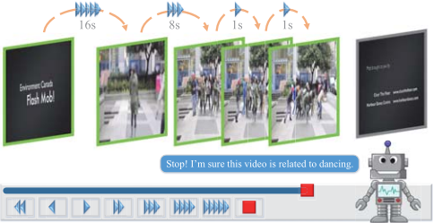
We evaluate our proposed efficient video classification model on the YouTube-8M [Abu-El-Haija et al., 2016] dataset, which is currently the largest video classification dataset. Compared to the models using all the video frames, our method effectively reduces the computation cost while maintaining the classification accuracy.
2 RelatedWorks
Video analysis: Many efforts have been made to improve video classification performance in recent years [Wang et al., 2011; Simonyan and Zisserman, 2014; Karpathy et al., 2014; Wang et al., 2016; Tran et al., 2015; Ng et al., 2015; Chang et al., 2016; Fan et al., 2017; Xu et al., 2015; Bhatnagar et al., 2017]. Video classification model generates representations which are usually beneficial to other video analysis tasks, i.e., video captioning [Pan et al., 2016] and video question answering [Zhu et al., 2017]. Hand-crafted features, especially Dense Trajectories [Wang et al., 2011; Wang and Schmid, 2013], can effectively represent short video clips but it is computational expensive. With the improvement of ConvNets models in image classification [Krizhevsky et al., 2012; Simonyan and Zisserman, 2015; Szegedy et al., 2016; He et al., 2016], deep models have also been proposed for video classification. Simonyan and Zisserman [Simonyan and Zisserman, 2014] first proposed to take stack optical flow images as inputs to a ConvNet. This two-streamConvNet, combining a rgb-net and a flow-net, outperforms improved Dense Trajectories [Wang and Schmid, 2013] on several action recognition datasets. Wang et al. [Wang et al., 2016] extended twostream ConvNet with a temporal segment network. Tran et al. [Tran et al., 2015; 2017] utilized 3D-ConvNets to model video spatio-temporal structures. Ng et al. [Ng et al., 2015] used an LSTM to aggregate frame-level ConvNet features for modeling video temporal sequences. Yeung et al. [Yeung et al., 2016] proposed a recurrent neural network-based agent for action detection. The agent interacts with the video globally, and there is no constraint on the action. We focus on video classification and limit our actions to a local range with a maximum step of 16s. The local pattern is then leveraged to predict what will happen in a short time. In this paper, we aim to improve video classification efficiency while retaining accuracy.
Reinforcement learning: Recently, deep reinforcement learning has made many breakthroughs in the field of artificial intelligence. On the aspect of computer vision applicatifons, Mnih et al.[Mnih et al., 2014] developed the recurrent visual attention model (RAM) which learns the spatial attention policies for image classification. Yeung et al.[Yeung et al., 2016] applied reinforcement learning to action detection.
3 Model
In this paper, we formulate our model into the reinforcement learning paradigm, which is about an agent interacting with an environment, and learning an optimal policy, by trial and error, for sequence decision making. We consider the 'fast forward' and 'adaptive stop' mechanisms as two sequential decision processes of a goal-driven agent interacting with a video player. At each time step, the agent is limited to observe only one frame from a video by a pre-trained ConvNet. However, the agent is capable of controlling which frame to be watched at the next time step or stop watching the video to emit classification decision at the current time step. The agent acts based on the current frame and history to watch the video efficiently. At the final step, the agent receives a scalar reward which depends on whether the classification decision is correct and the number of watched frames. The goal of the agent is to maximize such rewards.
3.1 Architecture
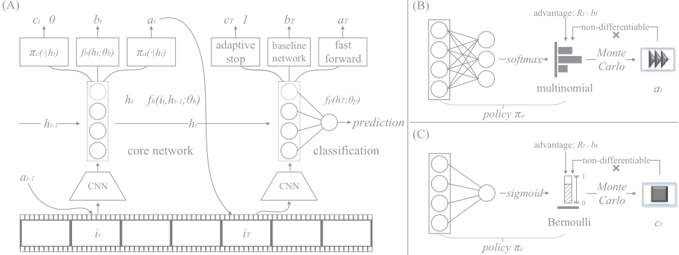
The agent is built around a core network as shown in Figure 2. At each time step t, the agent takes a frame feature it as input, integrates history information ht-1, and determines where to watch at at the next time step (fast forward network) or whether to stop watching ct (adaptive stop network) to make classification at the current step. When the agent decides to stop, a classification network is applied on the agent's internal state ht and emits the prediction p. We also add a baseline network to predict the expected return bt according to the current internal state, which is used to reduce variance during training [Williams, 1992].
Core network: The core network maintains an internal state which summarizes watching history information about the past frames; it encodes the agent's knowledge of the video and provides the information to guide the agent how to act at the next time step. The internal state ht at time t is formed by a recurrent neural network fh, which is parameterized by θh and updated over time with taking the external frame feature vector it as input ht = fh(ht-1, it; θh). The internal state ht plays a core role in the proposed approach. The fast forward action, adaptive stop action, baseline and classification decision are all based on this internal state.
Fast forward network: After observing a frame, the agent determine where to watch at the next time step by choosing an action at from a fast forward action space A. In this paper, the fast forward action space consists of seven discrete actions:
where '+' means forward and '-' means rewind. The motivation of this definition is that videos have local patterns, which can be learned and used to predict what will happen or appear within a few seconds. We premise that, exceeding 16 seconds, the pattern is too weak to be exploited. Therefore, we limit the agent to forward 16s at most at each time step. Sometimes, the agent may forward too much and miss information. To rescue this case, we add two rewind actions. However, we do not allow the agent to rewind too much because this would damage the efficiency. The agent should learn how to avoid over forward.
The fast forward network is implemented by a fully connected layer which is applied on ht, parameterized by θa, and followed by a softmax. This network outputs a multinomial probability distribution, i.e., the policy πa(·|ht; θa), which represents the probability of each action in A should be adopted. As shown in Figure 2(B), at is sampled from πa during training at ∼ πa(·|ht; θa). During evaluation, we use maximum a posteriori estimation to choose forward action, i.e., at = argmaxa πa(·|ht; θa).
Adaptive stop network: Adaptive stop is the other action which can be controlled by the agent. This action decides when to stop watching videos to begin classification. Unlike at, the adaptive stop action ct is a binary variable whose range is defined as:
In this paper, we use 0 to represent 'continue' and 1 to represent 'stop'. The adaptive stop network is a fully connected layer parameterized by θc and followed by a sigmoid, which takes ht as input and outputs a Bernoulli probability distribution, i.e., the policy πc(·|ht; θc), representing the probability of stop. As shown in Figure 2(B), ct is sampled from the πc during training ct ∼ πc(·|ht; θc)
Baseline network: To reduce variance during training, we use a baseline network to establish a baseline bt to encourage (if Rt > bt) or discourage (if Rt < bt) both the fast forward action at and adaptive stop action ct, where Rt is the return
(cumulative discounted reward) at the time step t with a discount factor γ ∈ (0, 1]: Rt = ∑T-t k=0 γ k rk+t. The baseline network is a linear regressor parameterized by θb and takes the core network's state ht as input bt = fb(ht; θb). The quantity Rt - bt, which is also called advantage, will be used to scale the policy gradients.
Classification network: When the adaptive stop is triggered, the classification network fp is applied on the final internal state hT . We consider a binary classification setting and train the agent for every class. Suppose the positive video is labeled as 1 and the negative video is labeled as 0, then fp outputs the likelihood p of the video to be positive. We use a fully connected layer parameterized by θp and followed by a sigmoid to predict the video label p = fp(hT ; θp), where T is the final time step which satisfies cT = 1.
Reward function: After classification, the agent receives a reward signal based on whether the prediction is correct and the number of watched frames. The goal of the agent is to maximize this reward. We denote the ground truth of the video label as g, the reward function is defined as follows:
When t = T, the reward function consists of two parts. The first one 1 - 2|p - g| is called accuracy reward, which depends on the correctness of prediction. Since p ∈ [0, 1] and g ∈ {0, 1}, this part maps the accuracy reward to [-1,+1]. The second part -μT is called frame penalty which is used to encourage the agent to watch less frames.
3.2 Training
The parameters of the agent consists of the parameters from the core network, fast forward network, adaptive stop network, baseline network and classification network, i.e., θ = {θh, θa, θc, θb, θp}. We use standard backpropagation to train fv, fp and REINFORCE to train πa, πc. The parameter of the core network θh is not directly optimized but can be updated by the gradients from the other four networks.
Classification loss: In this work, every agent focuses only on one specific video class. The output of the agent is a scalar variable with range [0, 1], which indicates the confidence score of a video example being positive. Therefore, we optimize the classification network parameter θp by minimizing the binary cross entropy loss:
Baseline loss: The baseline network fb is trained by minimizing the mean squared error loss:
At each training iteration, the fast forward network and adaptive stop network are first updated by the reward and the baseline. The baseline network is then optimized by Eq. (5). Note that this loss does not backpropagate to the fast forward network or the adaptive stop network.
Policy gradients: In this section, we derive the expressions for the parameter gradients for our setup. Recall that our agent takes two actions, i.e., fast forward action at and adaptive stop action ct at each time step. The objective of the agent is to maximize the reward rT achieved at the final step T:
Note that rt = 0 for t < T according to the reward function Eq. (3). The gradient of θa can be derived as follows:
As we can see from Eq. (7), the gradient ▽θa J is directly proportional to Rt. Updating the parameter directly according to Rt will make training very unstable. To reduce the variance of the gradient estimate, we subtract the baseline bt from Rt:
This is an unbiased estimation to the gradient because E πa,πc▽θa log πa(at|ht)bt = bt▽θa 1 = 0. Similarly, gradient
w.r.t. θc, i.e., ▽θc J can be derived as follows:
Since the dimension of the possible action sequence can be very high, it is impossible to optimize Eq. (8) and Eq. (9) directly. Following REINFORCE [Williams, 1992], we use Monte Carlo sampling to approximate the policy gradients. Encourage exploration: To avoid highly-peaked πa towards a few fast forward actions or a few fixed action sequences, which over-optimizes on a small portion of the environment, i.e., video in this work, we use an entropy term to encourage diversity [Mnih et al., 2016]:
When all actions almost have the same probability, the entropy will be high. Conversely, when one action has near 1 probability, the entropy will be low. Therefore, adding a negative entropy term to the loss function will penalize the actions that dominate the policy too quickly and encourage exploration.
Finally, our objective is to minimize the following hybrid loss function:
where α, β, λ and ρ are positive factors to control the weights of different sub-losses.
4 Experiments
4.1 Datasets and Settings
Since reinforcement learning usually needs large-scale datasets, we evaluate our method on the YouTube-8M [AbuEl-Haija et al., 2016] dataset, which is a large-scale video classification benchmark. YouTube-8M consists of ∼8 million videos - 500K hours of video, annotated with 4800 classes. The average length of the videos in the dataset is 230 seconds. In this paper, we select 20 classes from the 4800 visual entities to evaluate the proposed model. To collect videos, we first remove the the videos whose lengths are less than 16 seconds. For every class, we then randomly collect 10,000 positive videos and 40,000 negative videos for training, and 1,000 positive videos and 4,000 negative videos for evaluation. If the class contains less than 10,000 positive videos, we use all positive videos and still collect 40,000 negative videos. The videos in YouTube-8M are usually with multiple labels. When selecting negative videos, we simply guarantee the target class does not appear in them, meaning that the positive videos and negative videos may have some intersection labels. We report mean average precision (mAP) for all experiments.
| class | 5 | 10 | 15 | 30 |
|---|---|---|---|---|
| vehicle | 92.6 | 95.0 | 95.2 | 95.4 |
| video game | 88.6 | 90.0 | 90.2 | 90.4 |
| concert | 95.3 | 96.3 | 96.9 | 96.9 |
| car | 94.9 | 96.3 | 96.5 | 96.6 |
| dance | 89.2 | 90.1 | 90.2 | 90.3 |
4.2 Implementation Details
We decode videos at one frame per-second and extract features from the last hidden representation of Inception-v3 network [Szegedy et al., 2016] before the classification layer. The features are then normalized by ℓ2 normalization. The hidden state size of RNN is set to 128. Each agent is trained for 50 epochs. We set batch size to 32, dropout rate to 0.5 and gradient clipping to 5.0. We optimize our model with the Adam optimizer with a fixed the learning rate of 1×10⁻³ . We search for the reasonable values of α, β, λ and ρ in Eq. (11) on the vehicle class. We then fix α = 1.0, β = 0.5, λ = 1.0 and ρ = 0.01 in all experiments. The discount factor γ is 0.9.
4.3 Ablation Study
Fast forward network. To explore what policy the fast forward network learns, we set the frame penalty μ to 0 but force the agent to watch 5, 10, 15, and 30 frames in this experiment.
| class | μ = 10-1 | μ = 10-2 | μ = 10-3 | μ = 10-4 | ||||
|---|---|---|---|---|---|---|---|---|
| mAP# | framesmAP# | framesmAP# | framesmAP# | frames | ||||
| vehicle | 68.4 | 2.12 | 95.1 | 7.58 | 95.2 | 10.24 | 95.1 | 10.64 |
| video game | 62.0 | 1.91 | 90.2 | 7.84 | 90.4 | 9.04 | 90.4 | 9.25 |
| concert | 71.0 | 2.42 | 96.5 | 6.73 | 96.8 | 7.82 | 96.9 | 8.46 |
| car | 67.1 | 2.33 | 96.3 | 7.46 | 96.5 | 9.30 | 96.7 | 10.66 |
| dance | 60.7 | 1.88 | 90.1 | 6.69 | 90.5 | 7.99 | 90.6 | 9.01 |
We evaluate the fast forward mechanism on the vehicle, video game, concert, car and dance classes. The experiment results are listed in Table 1. Basically, when the number of frames allowed to be watched increases, the mAP improves. However, when the number of frames allowed to be watched exceeds 10, the mAP does not improve much.
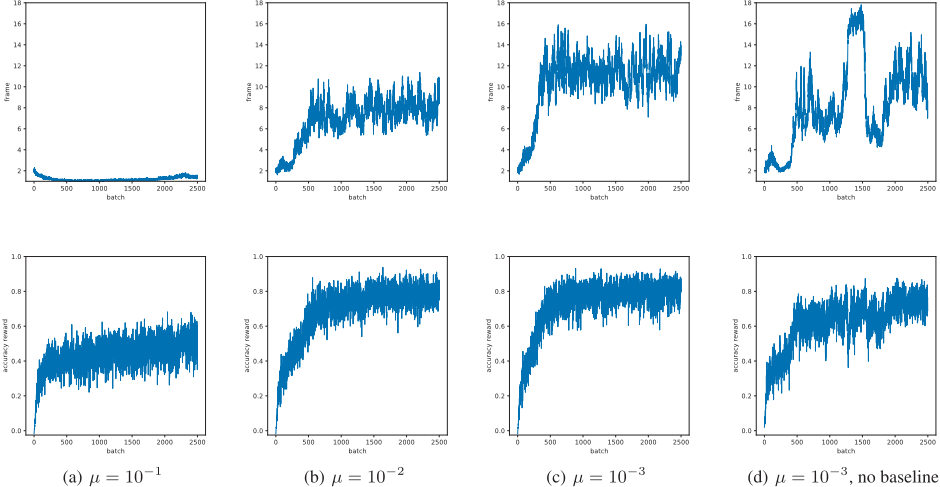
Adaptive stop network. The step penalty factor μ controls the number of frames the agent will see. Generally, a large μ can improve the efficiency for video classification but may damage the accuracy. In this section, we explore how the step penalty factor influences the behavior of the adaptive stop network. To this end, we select μ from {10-1 , 10-2 , 10-3 , 10-4 }. We record the average of used frames and the accuracy reward during training. We show the results of first 2,500 training batches in Figure 3.
When μ changes from 10-1 to 10-3 , the agent uses more and more video frames for classification. However, the accuracy reward do not increase when μ ≤ 10-2 , which indicates that increasing the number of watched frames may not always significantly improve the performance.
| Pooling Method | Recurrent Neural Network | Our Method | ||||||||||||||
|---|---|---|---|---|---|---|---|---|---|---|---|---|---|---|---|---|
| class | Max Pooling | Average Pooling | LSTM | GRU | RL-LSTM | RL-GRU | ||||||||||
| R10 | U10 | All | R10 | U10 | All | R10 | U10 | All | R10 | U10 | All | mAP | # frames | mAP | # frames | |
| vehicle | 88.3 | 86.3 | 83.1 | 93.4 | 93.2 | 94.7 | 93.7 | 93.7 | 94.8 | 94.1 | 93.9 | 95.5 | 94.2 | 5.68 | 95.1 | 7.58 |
| video game | 77.6 | 75.9 | 65.7 | 81.7 | 81.6 | 83.0 | 88.9 | 90.6 | 88.5 | 88.9 | 88.6 | 90.6 | 88.8 | 5.57 | 90.2 | 7.85 |
| concert | 93.3 | 91.1 | 88.3 | 94.8 | 94.6 | 95.1 | 96.0 | 97.0 | 96.6 | 96.2 | 96.0 | 97.0 | 96.3 | 5.17 | 96.5 | 6.73 |
| car | 92.4 | 90.5 | 87.6 | 94.8 | 94.7 | 95.3 | 95.8 | 95.5 | 96.4 | 95.6 | 95.1 | 96.6 | 95.7 | 7.57 | 96.3 | 7.45 |
| dance | 85.7 | 84.0 | 79.3 | 88.4 | 88.4 | 89.3 | 89.3 | 89.2 | 89.6 | 89.6 | 89.7 | 90.4 | 89.9 | 7.48 | 90.1 | 6.69 |
| animation | 82.9 | 80.2 | 76.1 | 86.8 | 86.9 | 87.8 | 88.6 | 88.3 | 88.9 | 89.1 | 88.8 | 90.1 | 88.5 | 5.54 | 90.2 | 8.33 |
| musician | 88.6 | 87.7 | 84.3 | 92.0 | 92.1 | 92.6 | 92.5 | 92.6 | 93.1 | 92.8 | 92.7 | 94.2 | 92.4 | 5.56 | 93.9 | 7.77 |
| music video | 73.0 | 71.5 | 64.6 | 78.0 | 77.7 | 80.5 | 82.2 | 82.5 | 84.9 | 83.5 | 83.1 | 87.7 | 83.1 | 5.83 | 87.3 | 7.08 |
| animal | 82.0 | 80.1 | 63.1 | 88.1 | 87.9 | 89.8 | 89.7 | 89.5 | 90.6 | 89.0 | 89.2 | 91.4 | 89.3 | 6.18 | 90.5 | 8.02 |
| album | 73.0 | 70.4 | 67.1 | 76.2 | 76.2 | 77.3 | 76.8 | 76.7 | 77.9 | 79.0 | 78.7 | 79.3 | 78.7 | 5.27 | 79.5 | 9.36 |
| medicine | 74.1 | 71.9 | 62.8 | 79.7 | 79.8 | 81.0 | 83.0 | 83.2 | 84.3 | 84.8 | 84.6 | 85.5 | 84.0 | 7.15 | 85.0 | 8.69 |
| kitchen | 94.1 | 93.0 | 88.3 | 95.4 | 95.2 | 95.3 | 95.2 | 95.0 | 96.1 | 95.5 | 95.2 | 96.6 | 94.8 | 5.38 | 95.9 | 9.01 |
| computer | 90.4 | 87.9 | 84.7 | 93.2 | 93.0 | 93.9 | 94.1 | 94.0 | 95.2 | 94.3 | 93.9 | 95.4 | 94.1 | 6.51 | 94.7 | 6.51 |
| Christmas | 65.6 | 64.3 | 49.3 | 71.7 | 71.8 | 73.2 | 74.0 | 74.3 | 76.2 | 76.1 | 76.5 | 78.4 | 74.9 | 5.85 | 77.2 | 7.71 |
| eating | 84.2 | 83.9 | 67.9 | 88.7 | 88.6 | 89.3 | 89.5 | 89.2 | 90.1 | 89.7 | 89.6 | 90.8 | 90.2 | 7.45 | 89.9 | 7.64 |
| first-person shooter | 87.6 | 85.9 | 79.3 | 89.8 | 89.5 | 90.8 | 91.1 | 90.3 | 92.2 | 91.3 | 91.1 | 92.8 | 91.9 | 5.47 | 92.5 | 8.75 |
| rain | 71.1 | 70.3 | 62.4 | 77.1 | 77.2 | 78.7 | 78.2 | 78.3 | 79.7 | 78.4 | 78.6 | 80.5 | 78.3 | 5.81 | 79.8 | 8.06 |
| champion | 63.7 | 62.9 | 58.1 | 68.9 | 69.0 | 70.2 | 72.4 | 72.4 | 73.1 | 73.0 | 73.1 | 75.6 | 72.6 | 7.02 | 74.1 | 7.84 |
| egg | 65.6 | 63.8 | 51.3 | 74.4 | 74.8 | 76.3 | 77.0 | 76.7 | 78.3 | 77.5 | 77.3 | 78.7 | 77.6 | 6.76 | 77.9 | 6.57 |
| village | 71.2 | 70.0 | 60.6 | 76.0 | 75.7 | 77.9 | 80.8 | 80.7 | 81.5 | 81.1 | 80.9 | 82.3 | 80.8 | 5.79 | 82.4 | 7.24 |
| mean | 80.2 | 78.6 | 71.2 | 84.5 | 84.4 | 85.6 | 86.4 | 86.5 | 87.9 | 87.0 | 86.8 | 88.5 | 86.8 | 6.15 | 88.0 | 7.74 |
We evaluate the influence of different μ on the classes vehicle, video game, concert, car and dance. The experiment results are shown in Table 2. Basically, when μ decreases, the number of frames to be watched increases. However, when μ ≤ 10-2 , the mAP is not significantly improved.
Dose the baseline network reduce variance? In this section, we explore whether the baseline network helps reduce variance during training. To remove the influence of baseline network, we set β in Eq. (10) to 0. The frame penalty μ is set to 10-3 . The video class we used is vehicle and the RNN is GRU. We show the average of frames to be used and the accuracy reward during the first 2,500 training batches in Figure 3(d). Compared with Figure 3(c), the training process without baseline network is considerably unstable, especially for the change of the amount of watched frames as shown in Figure 3(d). Therefore, replacing the return Rt by the advantage Rt-bt can significantly reduce variance during training.
4.4 Comparison with Other Methods
In this section, we compare our approach with other four methods, i.e., max pooling, average pooling, LSTM and GRU. For each method, we evaluate three cases: randomly sampling 10 frames (R10), uniformly sampling 10 frames (U10) and using all frames (All). For each model using random sampling, we evaluate three times and report the average results. For our approach, we set μ to 10-2 and both LSTM and GRU are evaluated. All 20 classes are used in this experiment. The results are listed in Table 3.
Compared with max pooling, average pooling, LSTM and GRU using 10 frames, Our method achieves the best performance. Especially for RL-GRU, it only uses 7.74 frames on average but acquire 88.0% mAP, which outperforms R10GRU by 1.0% and U10-GRU by 1.2%. RL-GRU also achieves very similar mAP to the All-GRU (88.5%). What is more, for some classes, RL-GRU even achieves better performance the All-GRU. Take the class album as an example, All-GRU achieves 79.3% while RL-GRU achieves 79.5% but only uses 9.36 frames on average. For the class village, AllGRU achieves 82.3% while RL-GRU achieves 82.4% using only 7.24 frames on average. This proves that our method is capable of achieving comparable and even better performance than using all frames.
Recall that the average length of videos in YouTube-8M is 230s and we decode videos at one frame per-second, which indicates that using all frames means using 230 frames on average. Our RL-GRU model achieves similar mAP to the AllGRU using only 7.74 frames on average, which significantly improves the classification efficiency.
5 Conclusion
We have proposed an agent that can make classification decision by watching temporally untrimmed videos efficiently. The agent has two mechanisms, i.e., "fast forward" and "adaptive stop" mechanism. We use REINFORCE to train the two mechanisms. By the "fast forward" and "adaptive stop" mechanisms, our agent significantly reduces the computational cost for video classification while maintaining the accuracy.
@inproceedings{ijcai2018p98,
  title     = {Watching a Small Portion could be as Good as Watching All: Towards Efficient Video Classification},
  author    = {Fan, Hehe and Xu, Zhongwen and Zhu, Linchao and Yan, Chenggang and Ge, Jianjun and Yang, Yi},
  booktitle = {Proceedings of the Twenty-Seventh International Joint Conference on
               Artificial Intelligence, {IJCAI-18}},
  publisher = {International Joint Conferences on Artificial Intelligence Organization},
  editor    = {Jérôme Lang},
  pages     = {705--711},
  year      = {2018},
  month     = {7},
  note      = {Main track},
  doi       = {10.24963/ijcai.2018/98},
  url       = {https://doi.org/10.24963/ijcai.2018/98},
}
TY - CPAPER TI - Watching a Small Portion could be as Good as Watching All: Towards Efficient Video Classification AU - Fan, Hehe AU - Xu, Zhongwen AU - Zhu, Linchao AU - Yan, Chenggang AU - Ge, Jianjun AU - Yang, Yi T2 - Proceedings of the Twenty-Seventh International Joint Conference on Artificial Intelligence, IJCAI-18 PB - International Joint Conferences on Artificial Intelligence Organization PY - 2018 SP - 705 EP - 711 DO - 10.24963/ijcai.2018/98 UR - https://doi.org/10.24963/ijcai.2018/98 ER -Copied
Machine-readable versions of this paper, for tools and AI agents:





