Mixed Causal Structure Discovery with Application to Prescriptive Pricing

1 Introduction

Prescriptive pricing [Caro and Gallien, 2012; Ito and Fujimaki, 2016; 2017] is one of the most advanced pricing techniques, which derives the optimal price strategy to maximize future profit/revenue on the basis of demand forecasting. Prescriptive pricing generally carries out a two stage analysis, 1) demand modeling that reveals the exact price-demand laws by discovering the quantitative causal relationships among prices, sales, and objective factors from historical observations, and 2) pricing optimization that finds the optimal price strategy by resolving a mathematical optimization problem constructed from the discovered relations. Demand modeling plays a vital role in pricing. A correct detection of actual factors affecting sales and an unbiased estimation of their quantitative effects by demand modeling, act as the foundation of the second stage, and decide whether pricing optimization can choose key control factors for optimal pricing. (biased relation estimates leads to sub-optimal pricing solutions.)

∗Equal contribution. Corresponding author: Liu Chunchen.

Several issues are crucial and should be resolved in demand modeling for practical usage. Firstly, factors involved in pricing usually comprise a mixture of discrete (e.g., season) and continuous variables (e.g., prices, sales), needing a technique that can process mixed data types jointly. Secondly, demand modeling requires an accurate recovery of the quantitative price-demand relations, which is the foundation to achieve optimal price strategy. Thirdly, the demand modeling process should be efficient so as to timely catch the insight from the fast-changing market, especially to support online pricing.

The causal models targeting at causal relation discovery is a nature selection for discovering price-demand laws, and have been attracting extensive attention recently. A causal model describes the demand as a causal effect of its own price, the prices of competing products, promotion, seasonality, and etc. But the widely used causal models are essentially regressions [Lee, 2011; Caro and Gallien, 2012; Ferreira et al., 2015]. Regression for correlation analysis is not causal discovery in nature, and pseudo causes are always reported due to confounders, leading to a low accuracy of price-demand relation recovery. Speaking concretely, correlation analysis will produce a high miss-hunting ratio of actual causes and much biased estimations of causal effects.

Causal structure discovery is able to eliminate pseudo causes by telling causation from correlation. Structural equation models (SEM) and causal Bayesian networks are two main classes of causal models [Pearl, 2009]. Recently, a family of SEMs called Causal Additive Noise Models (ANM) [Shimizu et al., 2011; B¨uhlmann et al., 2014] have been widely applied in causal structure discovery of continuous variables. ANM also can deal with discrete variables [Peters et al., 2011a], but the case involving a mix of continuous and discrete variables has received little attention. Causal Bayesian network gives a probabilistic interpretation of causal relations. Independencebased methods like PC [Spirtes et al., 2000] and score-based methods like GES [Chickering, 2003] are able to identify the causal graph from the joint distribution up to Markov equivalence, under the causal Markov condition and faithfulness condition [Pearl, 2009]. There has been a long line of work on recovering a hybrid Bayesian network from a mixture of variables by discretizing continuous variables [Monti and Cooper, 1998; Dojer, 2016], or converting the conditional distributions of all variables into the same type [Romero et al., 2006]. Until recently, some work [Cui et al., 2016; Sedgewick et al., 2017] adopted conditional independencebased methods to infer causal structures from mixed data.

In this paper, we develop a mixed causal model to describe price-demand relationships, propose a novel information criterion and derive related inference algorithms, to tackle the general issues required by demand modeling for practical usage. Our contributions can be detailed as follows:

Mixed causal model: We develop a mixed causal model for a mixture of discrete and continuous variables, and prove its identifiability in the bivariate cases.

Mixed information criterion: For score-based causal discovery, the key is an information criterion used for evaluating how mixed data fit a causal graph, which should be factorizable and tractable to compute. We derive a locally consistent criterion named Mixed Information Criterion (MIC) to tackle this problem.

Factorized causal inference: Based on MIC, we derive an inference framework for efficient structure discovery. Speaking concretely, with MIC, we construct a factorized optimization problem, on which an explorative search can be adopted to recover the causal structure. To accelerate the search process further, we propose ancestor-based search space cutting for speeding up without losing accuracy.

Evaluation on simuation/real retail datasets: We combine the proposed demand modeling technique with a latest pricing optimization method for test on both simulation and real datasets. Experiment results show that comparing with existing causal methods, our technique shows superiority in price-demand law recovery, supports demand prediction with higher accuracy, and helps to achieve higher gross profit.

2 Mixed Causal Modeling

Suppose we observe all factors relating to pricing, and have historical data X = [X1, · · · ,XD], where each random variable Xi can be binary (Xi ∈ {0, 1}N ), categorical (Xi ∈ {1, ..., T}N ), or continuous (Xi ∈ RN ). Since a categorical variable with T class can be translated to (T - 1) binary variables equally by standard practice, X is simplified as a mixture of binary and continuous variables. Under the causal markov and faithfulness assumptions, we model the relationships among the D observed variables as a probabilistic graphical model defined over a directed acyclic graph (DAG) G. Each random variable Xi corresponds to a node in G, and there is an edge linking fromXi to Xj if Xi is a direct cause of Xj . The probability graph model is in the form,

where Pa(Xi) is the parent set of Xi in G. pb(·) and pc(·) denotes the probability distribution of binary and continuous variables, respectively. zi ∈ {0, 1} is an indicator variable that zi = 1 if the variable Xi is binary and zi = 0 otherwise.

We assume the relations between a continuous variable and its parents are linear as (2) shows. Actually, the relations in real scenarios are generally non-linear, however, defining non-linear relations in demand modeling will raise great difficulty in the next pricing optimization stage, that is non-linear formulas make optimization problem hard to build and resolve or even lead the problem to be unsolvable. Alternatively, we represent non-linear by combining linear model and non-linear transformation of variables, which can avoid the above dilemma.

βi quantitatively describes the relations between Xi and all the other variables X-i where βij = 0 for Xj /∈ Pa(Xi). Here we use a symmetric super-Gaussian distribution, Laplace distribution, which will produce a least absolute deviation score that is robust to outliers, and has been reported work well in non-Gaussian causality estimation methods including LiNGAM [Hyv¨arinen and Smith, 2013], SLIM [Henao and Winther, 2011], and etc. We assume the relations between a binary variable and its parents as follows,

By introducing (2) and (3) to (1), we obtain the joint probability distribution,

where xin is the n-th element of Xi.

2.1 Identifiability of the Mixed Causal Model

Here we give the definition of bivariate identifiability and prove the above mixed causal model is bivariate identifiable.

Definition 1 (Bivariate Identifiability) [Peters et al., 2011b] Let F = {f|f : R2 → R} be a set of functions, PU = {PR,P{0,1}} denotes the set of probabilistic distributions for continuous/binary random variables, we call a set B ⊆ F × PU × PU containing functions f ∈ F and distributions of inputs X and noise ε bivariate identifiable in

holds. Additionally, we require f(X, εY ) ⊭ X for all (f, PX, PεY ) ∈ B with X ⊨ εY .

Theorem 1 For the mixed causal model, F = {fc, fb|fc(x, ε) = βx + ε, fb(x, ε) = { 1 βx+ ε > 0 0 otherwise }, PU is a set of non-Gaussian distributions with Laplace distribution for noise on continuous variables and Logistic distributions for noise on binary variables. The model is bivariate identifiability.

Here we provide an intuition rather than a formal proof which can be found in Appendix A. Briefly speaking, i) for the case that both variables are continuous, the model degenerates to a kind of linear ANMmodel of which the identifiability has been well proved by existing work [Shimizu et al., 2006]; ii) for the case that both variables are binary, with a sufficient condition that the random variables do not share the same marginal distribution, the model is identifiable; iii) for the case of a mixed of binary and continuous variables, based on the differences in conditional distributions, the model is identifiable.

3 Causal Inference

3.1 Mixed Information Criterion (MIC)

In the score-based causal inference approach, a scoring function is defined over the space of DAG, and one searches this space for a structure that optimize the scoring function. While the traditional approaches estimate the graph structure G and parameters {β1, . . . , βD} jointly using scoring functions like the Bayesian Dirichlet likelihood-equivalent (BDe) [Chickering, 2003], we propose a mixed information criterion (MIC), to assess the fit of a DAG on a mixture of binary and continuous variables, as follows,

where LL(Xi|Pa(Xi)) is the negative log-likelihood of data, and Pen(Xi, Pa(Xi) is the ℓ0 penalty. We introduce a scale parameter {wi}Di=1 to make the negative log-likelihood of different variables comparable in terms of magnitude. The magnitude of the negative log-likelihood changes a lot from one variable to another, especially when the observations are a mixture of binary and continuous variables. Such magnitude variation may comes from the differences in the value of variables which are measured on different scales. Normalization is one common way to adjust different variables to an aligned scale, but it might bring undesirable changes into the probability distribution of adjusted variables, which will lead to an accuracy loss of causal structure estimate. Our introduced scale parameter {wi}Di=1 is an alternative way for scale aligning while avoiding changing the data distribution. The magnitude variation may also comes from the estimation errors of model parameters, which will further bias the estimate of causal structure. Using a relative loss as MIC does is more robust to such magnitude variation than using an absolute loss if the scale parameter is proper designed. Here, we fix the value of wi to an underestimate of LL(Xi|Pa(Xi)), that is,

Pac(Xi) is the optimal potential parent set of variable Xi, and Pa(Xi) ⊆ Pac(Xi). The relative loss LL(Xi|Pa(Xi))/wi measures the ratio of the absolute loss to an optimistic estimate, and is robust to data scale variations and estimation errors as validated by the experiments.

We give the definition of local consistency and prove that MIC score is locally consistent. Local consistency, which was proposed in [Chickering, 2003], means that optimizing the model selection criterion leads to select a graph that can represent the data generating distribution, and the graph contains no edges that are redundant for representing the data generating distribution [Schulte and Gholami, 2017].

Definition 2 (Local Consistency) [Chickering, 2003] Let X be a set of data consisting of N records that are iid samples from some distribution p(·). Let G be any DAG, and let G ′ be the DAG that results from adding the edge Xi → Xj. A scoring criterion S(G, X) is locally consistent if the following two properties hold:

where, PaGj is shorten for Pa(Xj) in the DAG G.

Theorem 2 MIC score is locally consistent.

The formal proof can be found in Appendix B.

3.2 MIC-Based Causal Inference

With the new defined MIC used for evaluating the goodness of causal structures, we construct an optimization formulation to model the problem of causal structure discovery from mixed data. Speaking concretely, by instantiating the loglikelihood in (6) with the joint probability distribution in (4), we obtain a target for optimization, and a DAG constraint and ℓ0 constraints are added to achieve a sparse network.

S(βj) denotes the support set of βj. When resolving formula (9), the challenge is how to minimize an objective while enforcing the implied graph structure should contain no directed cycles. Existing researches [Koller and Friedman, 2009] show that the DAG-constraint structure learning problem can be cast as that of learning an optimal ordering of variables. Once the variable order is fixed, the constraint of no directed cycles can be enforced by constraining the parents of a variable to be a subset of variables ordering precede it. Binding with our case, we translate the problem in formula (9)

to a dynamic decision problem, of which the resolving will simultaneously produce the optimal variable ordering and a DAG-satisfied sparse causal structure.

U (U ⊆ X) is a set of variables of which the order have not been identified, orderSc(·) is the score of the optimal ordering of ·, nodeSc(·|¯·) is the optimal score of · under the choice of its parents from ¯·, Pac(Xj) is the optimal potential parent set for variable Xj, whose computation is described as formula (7). Take (X \ U) ∩ Pac(Xj) as candidate parents for computing nodeSc for Xj (formula (10)) will not reduce the causal discovery accuracy compared with using X \ U, but will save computation cost greatly (experiments show this further). We resolve the ℓ0 regression problems (11) by applying the forward backward greedy (FoBa) algorithm [Zhang, 2011] since it offers the tightest upper bounds of feature selection error, estimation error, and objective error. Although the upper bounds for the original FoBa algorithm have only been derived for least square regression, we can achieve the same bounds for our problem by slightly modifying the proofs of [Zhang, 2011]. Please refer to Appendix A for how we adapt FoBa to our problem.

A* FoBa for Optimization

For the dynamic decision problem like formula (10), some previous work [Xiang and Kim, 2013] solves it by finding a shortest path in the order search space. The start state of this order search space is an empty variable set, the goal state is the complete variable set, and any other state represents a subset of the complete variable set. In this order search space, an arc is always linking from one state to another with one more variable added. Each arc has been assigned a cost, and a path from start to goal with the lowest total cost is called the "shortest" path. The order according to which variables are added on the "shortest" path is the optimal variable order. We borrow the idea and derive our own method A* FoBa for the MIC-based causal inference. It is called A* FoBa because we resolve the optimization problem in (10) by A* search, and solve the sparse regression problems in (11) using FoBa algorithm. Start from the start state in the order space, A* search explores a shortest path, by greedy selecting the most promising succeeding state. A state Q is called most promising if its estimated cost, f(Q) = g(Q)+h(Q), is the lowest. g(Q) summarizes the cost of the arcs on the path from the start to the Q state, which denotes the cost incurred so far. h(Q) is the estimated future cost to be incurred from Q to the goal. Based on formula (10), we derive g(Q) and h(Q)

as following,

ΠQ denotes an ordering of the nodes in Q and ΠQ≺X denotes the set of variables in Q that precede X in ΠQ. A* search requires the h function to be admissible, meaning that h(Q) is always an underestimate of the true cost to reach the goal. Also, the h function should be consistent, meaning it should satisfy h(Q) ≤ c(Q, Q′ )+h(Q′ ), where Q′ = Q∪{Xj} is a succeeding state and c(Q, Q′ ) = nodeSc(Xj |Q∩P ac(Xj )) is the cost of moving from Q to Q′ . We prove that, based on score definitions((11), (13)) and the working process of the FoBa algorithm, h(Q) in (13) is admissible and consistent.

Theorem 3 The h function in equation (13) is admissible.

Proof: The true cost from the current state to the goal is T(Q) = ∑X∈X\Q nodeSc(X|Π≺X ∩ Pac(X)). The parent set selected by nodeSc(X|X \ X) in h is Pac(X) based on the definition in (7), while the parent set selected by nodeSc(X|Π≺X ∩ Pac(X)) is a subset of Pac(X) and denoted by Pa′c (X). Considering the feature selection process of FoBa, a feature r ∈ Pac(X) \ Pa′c (X) will be selected only if nodeSc gets smaller. Therefore, h(Q) ≤ T(Q) and the h function is admissiable.

Theorem 4 The h function in equation (13) is consistent.

Based on Theorem 1, Theorem 2 can be easily proved, and we skip it because of the space constraint.

3.3 Ancestor-Based Search Space Cutting

We utilize the ancestor relations to further cut down the order search space for inference accelerating.

Theorem 5 Ancestor relations can be used to prune the search space without losing optimality.

Proof: Given Q the set of variables assigned in the current state, and Q ∩ {Xi,Xj} = ∅, there are two paths to achieve the future state with variables Q ∪ {Xi,Xj}. Path1 is Q → Q∪ {Xi} → Q∪ {Xi,Xj}, and Path2 is Q → Q∪ {Xj} → Q∪ {Xi,Xj}. If the ancestor relation between two variables, e.g. Xi ≺ Xj, is known, then we can eliminate Path2 because it is always suboptimal compared with Path1 which is proved as follows,

in which nodeSc(Xi | Q∪{Xj}∩Pac(Xi))=nodeSc(Xi | Q ∩ Pac(Xi)) due to the ancestor constraint Xi ≺ Xj .

Algorithm 1 A* FoBa with ancestor-based space cutting

Input: Data X, the number of variables D

Output: Optimal structure B = {βd}Dd=1

Initialize:empty queue open, empty set close

• 1: For each variable Xj ∈ X, get its optimal potential parent set Pac(Xj) by solving (7) using FoBa
• 2: Construct an adjacent matrix from {Pac(Xj)}Dj=1
• 3: Extract m SCCs of variables scc1 ≺ scc2 ≺ · · · ≺ sccm from the adjacent matrix using Tarjan's algorithm [Tarjan, 1972]
• 4: Project SCCs onto a series ordering constraints C = {Xi ≺ Xj | Xi ∈ scck,Xj ∈ sccl, scck ≺ sccl}, ∀i, j ∈ {1, · · · ,D},∀k, l ∈ {1, · · · ,m}
• 5: open.insert(Q= ∅, f(∅) = h(∅), g(∅) = 0,BQ = ∅) 6: while true do 7: Q, f(Q), g(Q),BQ ←open.pop() 8: if h(Q) = 0 then return BQ end if 9: for each Xj ∈ X \ Q do 10: Q′ ←Q∪ {Xj} 11: if Q′ /∈ close and not voilate(Q′ ,C) then 12: Compute nodeSc(Xj | Q∩Pac(Xj)) by (11) 13: g(Q′ ) ← g(Q) +nodeSc(Xj | Q∩Pac(Xj)) 14: h(Q′ ) ← h(Q) -nodeSc(Xj | X \Xj)) 15: f (Q′ ) ← g(Q′ ) + h(Q′ ), BQ′ ← BQ ∪ {βj} 16: open.insert(Q′ , f (Q′ ), g(Q′ ), BQ′ ) 17: close ← close ∪{Q′ } 18: end if 19: end for
• 20: end while

We first learn the ancestor relations among all the variables, and then project these ancestor relations onto a series of topological ordering constraints, which can be easily integrated into the A* FoBa framework for search space cutting. The whole algorithm is summarized in Algorithm 1. The function voilate(Q′ ,C) in line 11 checks whether the current variable ordering violates the topological ordering constraints. The time complexity of our MIC-based causal inference algorithm is O(mmaxi 2|scci|D2N), where m is the number of strongly connected components (SCCs) [Tarjan, 1972], |scci| is the number of variables in the SCC scci, D denotes the total number of variables, N is the sample number.

4 Simulated Study

4.1 Synthetic Data

We simulated prices and sales of 40 kinds of beer, and 9 objective factors (i.e., temperature (continuous), seasonality (4, binary), vacation (binary), promotion (binary) and sunny/rainy (2, binary)). We used ptm and qtm to denote the price and sales of the m-th product in the t-th day, and denoted the n-th objective factor in the t-th day as gtn . To mimic the nonlinear relations between prices and sales, we introduced univariate transformation on prices that are f1 (ptm) = 1/ptm, f2 (ptm) = ptm, and f3 (ptm) = ln (ptm). Prices and sales are simulated by (15) and (16). The coefficient {α∗ , β∗ , γ ∗ , a∗ , b∗ , c∗ } were randomly generated from reasonable ranges. For noisy terms ϵ or e, we simulated exponential distribution and mixture Gaussian distribution.

We simulated 16 experiment settings differed in noise types, sparsity (simple/complex structure), train sample scale (1/3 years), and test sample scale (7/30 days). b∗ = 0 holds in the simple structure, while b∗ is not zero in complex structure. Under each setting, we generated 10 datasets while each contained 169 random variables.

4.2 Benchmarks

We compared our method with 7 other methods, 1) the l0 sparse regression [Liu et al., 2014] as a representative of regression-based demand modeling, 2) stable PC [Colombo and Maathuis, 2014] that is an improved version of the classical constraint-based method, PC, 3) causalMGM [Sedgewick et al., 2017], which is a latest constraint-based method for mixed data processing, 4) GES [Chickering, 2003] that is a classical score-based method, 5) A* Lasso [Xiang and Kim, 2013] whose shortest path finding framework we refer to, 6) Direct LiNGAM [Shimizu et al., 2011] that is designed for linear non-Gaussian data, 7) CAM [B¨uhlmann et al., 2014] that is a nonlinear-Gaussian SEM. Besides implementing the l0 sparse regression by ourselves, we used the implementations provided by authors and their default parameter settings for all the other benchmarks. The stable PC and causalMGM use the likelihood ration test (LRT) for independent test.

4.3 EvaluationMetrics

We consider the following evaluations:

Causal structure discovery (price-demand law discovery): Two metrics were used to measure the accuracy of structure discovery: 1) Precision = TP TP+FP , denoting among all the discovered causal relations, how many actually hold, and 2) Recall = TP TP+FN , denoting among all the actual causal relations, how many have been identified.

Demand forecasting: We used the learnt demand models to predict sales of 40 products on the test samples, and we used the averaged root-mean-square error (RMSE) to measure the prediction accuracy.

Pricing strategy: Based on a learnt demand model, we defined the optimization target, gross profit, as

where p = {pm}Mm=1 are control variables to be optimized, g = {gn}Nn=1 are external variables whose values are already known from test samples. qtm(·) is the function revealing price-demand relations. T is the number of test samples, rm is the cost of the m-th product. With the gross profit function as objective and with some actual requirements as constraints

(e.g., pm is chosen from discrete values {pm1, . . . , pmJ}.), the pricing optimization problem was formulated as binary quadratic programming (BQP), and solved by a semi-definite programming (SDP) relaxation [Ito and Fujimaki, 2017].

For evaluation, let l∗ (·) denotes a gross profit function with true parameters {α∗ , β∗ , γ ∗ , a∗ , b∗ , c∗ }, then the true optimal pricing strategy is p∗ = argmaxp l∗ (p). Let ˆl(·) denotes a profit function on { ˆα, ˆβ, ˆγ, ˆa, ˆb, ˆc} that are learnt by a demand model from train data, then a generated pricing strategy is ˆp = argmaxp ˆl(p). We used l∗ (ˆp) l∗ (p∗ ) ∈ [0, 1] to measure the goodness of a pricing strategy. (l∗ (ˆp) means the actual profit if running strategy ˆp in real environments, while l∗ (p∗ ) means the ideal profit if using optimal strategy p∗ .)

4.4 Experimental Results

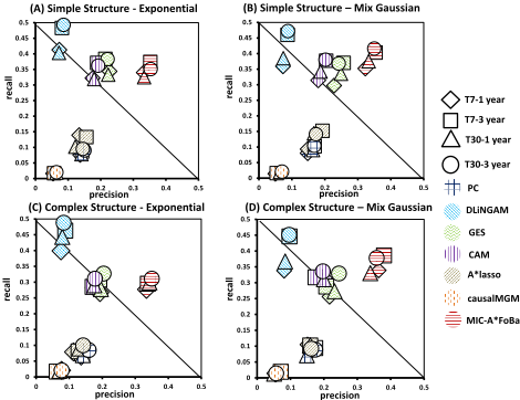
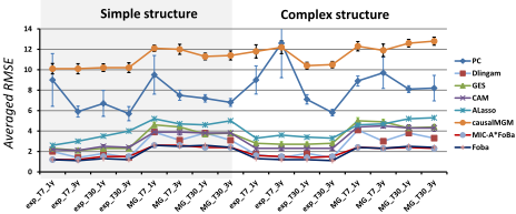
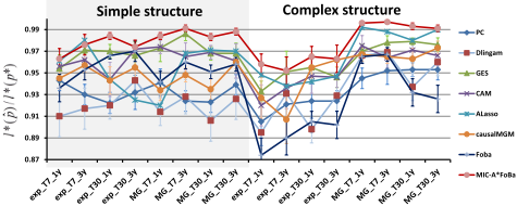
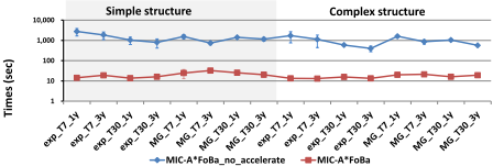
Figure 1 summarizes the accuracy comparisons for causal structure discovery. The four sub-figures tell us that, across all the datasets that vary in structure, noise distribution, train data scale, and test duration, our method (MIC-A*FoBa) outperformed all the other methods in Precision obviously and identically. Such results mean that the causal relations detected by our method are more reliable since a higher ratio of its identified relations are actually true. When checking the performance of Recall, we find that our method is better than (Figure 1 B/D) or comparable with (Figure 1 A/C) most of the benchmarks except the DLiNGAM. A high Recall while a low Precision like DLiNGAM means that it hunts a large amount of true and pseudo relations at the same time, which is bad news especially for the pricing optimization, because these pseudo causes will bias the causal effects of true causes which will further lead to bad pricing strategy.

Figure 2 compares the demand forecasting accuracy. Results show that MIC-A*FoBa defeats all the other causal methods across all the datasets and achieved the smallest prediction error. Comparing MIC-A*FoBa with FoBa that is for prediction, they show comparable accuracy, which further confirms that the causal relations and their related causal effects learnt by MIC-A*FoBa is close to the groundtruth.

Figure 3 compares the goodness of pricing strategies. MIC-A*FoBa shows the best performance across all datasets, meaning that it helps to produce pricing strategies that bring the highest gross profits. For the l0 regression, it worked relative well on datasets with simple structures, but dropped sharply on complex structures. One possible explanation is that, the regression failed to find real causes for demand variation due to price interactions in complex structure, and such pseudo causes lead to produce sub-optimal pricing strategy.

In A*FoBa, we adopted two policies for accelerating the inference. One is by the ancestor-based search space cutting strategy, and the other is by adding Pac(·) to constraint the candidate parent space as the underlined part in formula (9) shows. We compare two versions of MIC-A*FoBa, one is with the above strategies adopted while the other does not. The comparison showed in Figure 4 confirms the usefulness of the policies for inference accelerating.

5 Real World Retail Data

5.1 Data and Experimental Settings

We applied our method to real retail data from a supermarket in Tokyo. 1 We used daily prices, univariate transformations on prices and sales of 10 products (5 kinds of milk and 5 kinds of bread) 2 in two years from 2012/01 to 2013/12. In addition, objective factors during the same period were used, like the daily guest flow volume (continuous), seasonality (4, binary), month (12, binary), weekend (binary), day of the week (7, binary), weather (binary), and temperature (continuous). In total, we used 69 randomly variables for analysis.

1 The data is provided by KSP-SP Co.,LTD.

We simulated the whole procedure of prescriptive pricing on this real data. For demand modeling, we learnt the sales formula of each product from the data of the year 2012. As for the price optimization, we constructed the optimization target, ˆl(p), using (17) setting the cost to 0 for simplicity, and then obtained a pricing strategy ˆp by maximizing the revenue. To evaluate the pricing strategy, we built an independent validation environment ˆl′ (·) by estimating new sale formulas on data from 2013/01 to 2013/09. Compared to ˆl(·), ˆl′ (·) is an environment that is more similar to the real one in the validation stage (2013/10). We ran the pricing strategy ˆp on data from 2013/10, and achieved ˆl′ (ˆp) as the validation revenue explained as running ˆp in the validation sale environment.

5.2 Causal-Structure-Based Insight

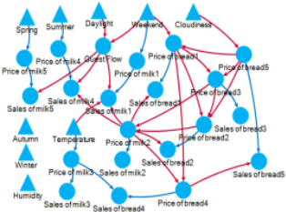
A subgraph of the causal graph learnt by our method was shown in Figure 5 to make a concise presentation. It illustrates some laws of market, such as the price elasticity of demand (e.g. price of bread1 has a negative effect on sales of bread1), the cross-price elasticity of demand (e.g. price of milk2 has a positive effect on sales of milk1). It also reveals some relations that are in accord with common sense, such as the guest flow has a positive effect on sales, and the weekend and daylight have a positive effect on guest flow.

5.3 Improvement of Profit

Figure 6 a ∼ c compare the predicted sales of different methods with the true sales, we find the predicted sales curves of Dlingam, Alasso, PC and CAM are much biased from the true ones, indicating they discovered pseudo causes and/or biased causal effects. Figure 6 d compares the validation revenue by different methods with the actual revenue computed from historical data (the above 4 methods are excluded because they performed not good at pricing and for a clear visualization.).

2 We used a few products to make causal graph visible and clear.

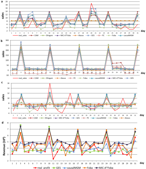
The sum of the validation revenue by GES, causalMGM, Foba, and MIC-A*Foba were 1.27×107 , 1.26×107 , 1.44×107 , and 1.58 × 107 respectively. The revenue obtained by our method is the highest. When comparing the curve of MICA*Foba with actual one in detail, we find that the improvements of revenue in low-actual-revenue days is more significant than that in high-actual-revenue days. It suggests that our pricing strategy is more effective when the business is tepid.

6 Conclusion

We proposed a mixed information criterion MIC and derived an MIC-based causal inference method for accurate causal discovery on mixed factor space. Experiments showed our demand modeling method outperformed other competitors in terms of causal recovery, prediction and pricing strategy.

A Proof of Bivariate Identifiability

We respectively prove the bivariate identifiability of mixed causal model in the binary-binary case, continuous-binary case, continuous-continuous case.

Theorem 6 Given a pair of binary variables (X, Y ) all of which take values in {0, 1}, under the mild assumption that X and Y do not share the same marginal distribution, the mixed causal model is bivariate identifiable.

Proof: If the mixed causal model is not bivariate identifiable, under the definition of the causal model and the definition of bivariate identifiability, there exist two models,

of which the joint distributions are the same. Let us consider their joint distributions respectively, that are,

If PM1 (X, Y ) = PM2 (X, Y ) holds, it induces that PM1 (X=0,Y =0) PM2 (X=0,Y=0) = 1, and it further induces k1 = k2, which conflicts with the assumption that the marginal distributions for X and Y should not be the same, so comes the theorem.

Theorem 7 Given a pair of mixed variables (X, Y ) that X takes value in R and Y takes value in {0, 1}, the mixed causal model is bivariate identifiable.

Proof: If the mixed causal model is not bivariate identifiable, under the definition of the causal model and the definition of bivariate identifiability, there exist two models,

of which the joint distributions are the same.

However, for model M1, we have P(Y = 1|X = x) = PεY (εY > -β1X) and PεY = logistic(0, 1), then

For model M2, from PεX = Laplace(0, b) and

which conflicts with that in (18), so comes the theorem.

Theorem 8 Given a pair of continuous variables (X, Y ) which all take values in R, the mixed causal model is bivariate identifiable.

Proof: For the situation where both variables are continuous, our model degenerate to a kind of linear additive noise model, whose identifiability has been well proved by [Shimizu et al., 2006].

B Proof of Local Consistency

Revisit the definition of decomposable MIC score in (6), ∣∣P aGj ∣∣ is the cardinality of PaGj ,

and BIC score is as follows,

Let X be a set of data consisting of N records that are iid samples from some distribution p(·). Let G be any DAG, and let G ′ be the DAG that results from adding the edge Xi → Xj ,

1. If Xj ⊭ pXi | PaGj ,

As BIC score is locally consistent [Chickering, 2003], BIC(G,X) - BIC(G ′ ,X) < 0 follows the definition of local consistency, wj, λ ∈ R+ are constant, logN → +∞ as N → +∞.

1. If Xj ⊨ pXi | PaGj ,

and thus,

Hence MIC score is locally consistent.