Estimation with Incomplete Data: The Linear Case

1 Introduction

Incomplete (or missing) data are data in which values of one or more variables are missing. Almost all existing techniques for handling incomplete data employ maximum likelihood or multiple imputation methods to fill in the missing values and estimate parameters of interest. To guarantee convergence and consistency, these techniques require that the missing data mechanism be ignorable ([Rubin, 1976]) i.e. the causes of missingness be either random or fully observed.

In practice, however, missingness is almost always caused by variables that are themselves afflicted by missingness ([Osborne, 2014; Sverdlov, 2015; Adams, 2007; van Stein and Kowalczyk, 2016]). Such data are called Missing Not At Random (MNAR). Among all MNAR problems, the most frequently encountered case is that of a variable causing its own missingness which we call self-masking MNAR. It is discussed in almost all literature on missing data including [Koller and Friedman, 2009] (chapter 19) and [Darwiche, 2009] (chapter 17). Examples include smokers not answering questions about their smoking behavior in insurance applications, longitudinal studies with attrition ([Little, 1995]), people with high income not revealing their incomes and a general reluctance to answer questions about sensitive topics such as religion, sexual preference and abortion ([Greenland and Finkle, 1995]).

While there has been some recent work ([Daniel et al., 2012; Mohan et al., 2013; Mohan and Pearl, 2014a; Mohan and Pearl, 2018; Thoemmes and Mohan, 2015; Shpitser et al., 2015]) on estimation in MNAR data with discrete variables, to the best of our knowledge there exists no theoretically sound and empirically efficient graph based procedure for handling MNAR missingness in datasets with continuous variables.

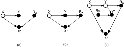
In this paper we focus on MNAR problems in linear systems. As in [Mohan and Pearl, 2014b] and [Mohan and Pearl, 2018], we treat missing data as a causal inference problem. We present sound, graph-based procedures for recovering (i.e. consistently estimating) parameters such as mean, variance and covariance. In the following section we review missingness graphs and structural equation models.

2 Preliminaries

2.1 Missingness Graphs: Notations and Terminology

Let G(V,E) be the causal DAG where V = Vo ∪ Vm ∪ U ∪ V ∗ ∪R. Nodes in the graph correspond to variables in the data set. E is the set of edges in the DAG. Vo is the set of variables that are observed in all records in the population and Vm is the set of variables that have missing values in at least one record. Variable X is termed as fully observed if X ∈ Vo and partially observed if X ∈ Vm. Rvi and V ∗ i are two variables associated with every partially observed variable, where V ∗ i is a proxy variable that is actually observed, and Rvi represents the status of the causal mechanism responsible for the missingness of V ∗ i ; formally,

V ∗ is the set of all proxy variables and R is the set of all missingness mechanisms. U is the set of unobserved nodes (or latent variables). We use bi-directed edges as a shorthand notation to denote the existence of a U variable as common parent of two variables in Vo ∪ Vm ∪R. For any W ⊆ Vo, Rw = ∅. Unless stated otherwise it is assumed that no variable in V ∪ U is a child of an R variable. This graphical representation is called Missingness Graph (or m-graph) ([Mohan et al., 2013]). An m-graph portrays Missing Completely At Random (MCAR) missingness if (Vm, Vo, U)⊥⊥R, Missing At Random (MAR) if (Vm,U)⊥⊥R|Vo and Missing Not At Random (MNAR) if neither MAR nor MCAR hold. Figure 1 (a), (b) and (c) exemplify MCAR, MAR and MNAR missingness respectively.

Proxy variables may not always be explicitly shown in mgraphs in order to keep the figures simple and clear. Conditional Independencies are read off the graph using the dseparation 1 criterion [Pearl, 2009]. Before formally defining the linear missingness model, we shall briefly review Structural Equation Models. For a detailed discussion see [Pearl, 2009] (chapter 5) and [Brito, 2004].

2.2 Structural EquationModels

A structural equation model (SEM) is a system of equations defined over a set of variables, such that each variable appears on the left hand side of at most one equation. Each equation describes the dependence of one variable in terms of the others and contains an error term to account for the influence of unobserved factors. Example: X = ϵx and Y = αX + ϵy. As in [Pearl, 2013], we interpret structural equations as an assignment process whose directionality is captured by a path diagram (see Figure 2). In this work all substantive variables ({Vm ∪ Vo ∪ U}) and error terms are assumed to be drawn from a Gaussian distribution. Linear Structural Equation Modeling is widely used for estimating parameters of interest given data that are missing at random ([Allison, 2003; Graham, 2003; Ullman and Bentler, 2003; Enders, 2006; Schlomer et al., 2010]).

2.3 Recoverability

Definition 1 (Recoverability of target quantity Q ([Mohan et al., 2013])). Let A denote the set of assumptions about the data generation process and let Q be any functional of the underlying distribution P (Vm, VO, R). Q is recoverable if there exists an algorithm that computes a consistent estimate of Q for all strictly positive manifest distributions P(V ∗ , Vo,R) that may be generated under A.

We present an example of recoverability in linear models in section 3.1. For examples of recoverability in nonparametric models with discrete variables, please see [Mohan et al., 2013].

3 Quasi-linear Missingness Model

The causal missingness mechanism is a binary variable and as such the function generating it cannot be linear. The quasilinear model defined below captures the missingness process.

1 For a quick introduction to d-separation see, http://www.dagitty.net/learn/dsep/index.html

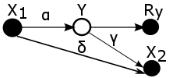
Figure 2: Quasi-linear missingness model and equations constituting the SEM corresponding to it.

Definition 2. A Quasi-linear Missingness Model is a Structural Equation Model such that:

1. every substantive variable X is a linear function of its causes ,Y , and a random error term ϵx

The coefficient α's are called path coefficients or structural parameters.

1. For every Rx ∈ R, Rx = f(Z, ϵRx ) where Z is the set of causes and f is a non-linear function. No R variable is a parent of any substantive variable.
2. Every proxy variable X∗ is generated by the non-linear function: X∗ = (1 - Rx)X + mRx

Figure 2 and equations (i) to (v) exemplify an m-graph and its corresponding quasi-linear missingness model. Path coefficients can be identified in linear models by applying criteria such as single door and back door (see [Pearl, 2009] (chapter 5)). In the following lemma we rephrase and state a basic result in linear path analysis that links covariance with path coefficients ([Pearl, 2013; Pearl, 2009; Brito, 2004; Wright, 1921]).

Lemma 1. Let G be an m-graph with k unblocked paths p1, ..pk between X and Y . Let Api be the ancestor of all nodes on path pi. Let the number of nodes on pi be npi .

where npi -1 ∏ j=1 αpi j is the product of all causal parameters on

path pi.

For example, in figure 2, there exist two paths, X1 → Y → X2 and X1 → X2, between X1 and X2. On applying lemma 1 we get, cov(X1, X2) = αγvar(X1) + δvar(X1).

In the following subsection we will exemplify a novel path analytic procedure for consistent estimation of the covariance matrix given MAR data.

3.1 Recoverability of Covariance Matrix: An Example

For any target quantity Qwe use Q‖RX=0 to denote: compute Q from samples in which all variables in X are observed.

Example 1. Consider the problem of estimating the covariance matrix given the MAR model of Figure 1 (b). Y is fully observed and hence var(Y ) is trivially recoverable. In order to recover cov(X, Y ), we will first recover βXY , the regression coefficient of X on Y . Since X⊥⊥Rx|Y we have the license to compute βXY (using OLS) from samples in which X is observed i.e. βXY = βXY ‖Rx=0 . cov(X, Y ) can now be recovered as:

• Recovering var(E(X|Y )): E(X|Y ) = βXY Y + cx where βXY and cx denote the slope and intercept of the regression line. Since X⊥⊥Rx|Y , E(X|Y ) = E(X|Y )‖RX=0 . Therefore,

• Recovering E(var(X|Y )): The variance of a conditional gaussian distribution is constant. Therefore,

Variance of a conditional bivariate Gaussian distribution, var(X|Y ), is given by var(X)(1 - ρ2 ), where ρ = cov(X,Y ) (var(X)var(Y )) 12 denotes the correlation coefficient. Since X⊥⊥Rx|Y , var(X|Y ) = var(X|Y )‖RX=0 . Hence,

Note that while all factors in the preceding estimand, except var(Y ) are estimated from samples in which X is observed, var(Y ) is recovered from all samples in the dataset, including those in which X is missing. In other words, although a consistent estimate of var(X) cannot be computed directly from fully observed data (i.e. P(X∗ , Y,Rx = 0)), it can be recovered by a procedure in which each factor in the estimand is estimated from subsets of the available data.

We further note that as a consequence of recovering var(X), βYX, the causal effect of X on Y can be recovered as,

The following section presents procedures for computing parameters of interest in quasi linear models.

4 RecoveringMean, Variance and Covariance

Theorem 1 (Recovering Mean of Partially Observed Variables). Let {X,Z} ⊆ Vm ∪ Vo, X ∩ Z = ∅, |X| = 1. Given m-graph G, E(X) is recoverable if there exists Z = {Z1,Z2, ...Zn} such that X⊥⊥RxRz|Z and E(Zi) is recoverable for all Zi ∈ Z. If recoverable, E(X) is given by

where c and αi's denote the intercept and coefficients of the regression line of X on Z.

Proof. Let X = α1Z1 + α2Z2 + ... + αnZn + c be the regression line of X on Z. Since X⊥⊥RxRz|Z, E(X|Z) = E(X|Z)‖Rxz=0 . Hence,

However since E(X) = E(E(X|Z)) we can write,

Theorem 2 (Recovering covariance of X and Y ). Let {X, Y,Z} ⊆ Vm ∪ Vo, X ∩ Y ∩ Z = ∅, |X| = 1, |Y | = 1 and |Z| = n. Given m-graph G, cov(Y,X) is recoverable if there exists Z = {Z1,Z2, ...Zn} such that (i) Y⊥⊥Rx,Ry,Rz|X,Z, and (ii) E(X),E(Y ), var(X), and ∀i E(Zi) and cov(X,Zi) are recoverable. If recoverable, cov(Y,X) is given by

where c and α's denote the intercept and coefficients of the regression line of Y on X, Z.

Proof.

Using Y ⊥⊥Rx, Ry , Rz |X, Z, we get E(Y |X, Z) = E(Y |X, Z)‖Rxyz=0 . Therefore,

A well known and widely used property of Gaussian distributions is that their conditional variances are constant. Let |X| = m and |Y | = n. Let Mxx,Myy and Mxy denote the covariance matrix of X, Y and X and Y respectively. Variance of the conditional Gaussian distribution f (Y |X) is given by,

Theorem 3 (Recovering variance of a partially observed variable X). Let {X,Z} ⊆ Vm ∪ Vo, X ∩ Z = ∅, |X| = 1 and |Z| = n. Given m-graph G, var(X) is recoverable if there exists Z = {Z1, Z2, ...Zn} such that X⊥⊥RxRz|Z and cov(Zi, Zj) is recoverable for all Zi, Zj ∈ Z. If recoverable, var(X) is given by

where αi's denote the coefficients of the regression line of X on Z.

Proof. We first apply the law of total variance: var(X) = E(var(X|Z)) + var(E(X|Z)), and then prove recoverability of var(X) by showing that both summands are recoverable.

Recovering E(var(X|Z)): Since X and Zi ∈ Z, ∀i are Gaussian variables, var(X|Z) is constant; therefore,

Recovering var(E(X|Z)): Since X⊥⊥Rx, Rz|Z we have,

Lemma 2. [Recovering Partial Regression Coefficients] Let {X, Y,Z} ⊆ Vo ∪ Vm. Given m-graph G and missing data D, partial regression coefficient βXY.Z is recoverable if X⊥⊥RX, RY , RZ|Y, Z and is given by βXY.Z‖Rxyz=0 .

Notice that recoverability of E(X) using theorem 1 is contingent upon the recoverability of E(Zi), for all i. Clearly, to recover E(X) we should recover all E(Zi)'s first. Similar is the case with theorems 2 and 3. In the case of recoverability of conditional distributions in datasets with discrete variables, [Mohan et al., 2013] defined the notion of ordered factorization to sequence the recoverability procedure. In the following theorem we adapt the idea of ordered factorization in [Mohan et al., 2013] to formulate a sufficient condition for recovering mean.

Theorem 4. Let Y ∪{Z} ⊆ Vm∪Vo and let O: Y1 < Y2 < . . . < Z = Yk be an ordered set of all variables in Y ∪ {Z}. Let Xi ⊆ {Y1, . . . , Yi-1}, 1 ≤ i ≤ k.

Given an m-graph G, a sufficient condition for recovering E(Z) is that there exist O and Xi ∀i such that Yi⊥⊥(Ryi , Rxi )|Xi .

Proof. Recoverability follows from theorem 1. We proceed by first recovering E(Y1) and then recovering E(Y2),..,E(Yk) sequentially in the order dictated by O.

Example 2. Consider the problem of recovering E(X) and E(Y ) given the m-graph G in figure 1 (c) and ordering O : Y < X. Ordering O directs us to first recover E(Y ) and then recover E(X). Since Y⊥⊥Ry in G, we can apply theorem 1 to recover E(Y ) as E(Y )‖Ry=0 . Since X⊥⊥Rx, Ry|Y and E(Y ) is recoverable, we can apply theorem 1 to recover E(X) as c‖Rxy=0 + α1‖Rxy=0 E(Y )‖Ry=0 .

In a similar manner, ordered recoverability procedures can be extended to recover covariance and variance as well. In the case of MCAR data, all orderings of variables will guarantee recoverability, whereas in the case of MAR data, orderings in which all fully observed variables precede partially observed variables will guarantee recoverability. Finally in the case of MNAR data, the ordering is determined by graph structure, and heuristics for finding admissible orders are discussed in [Mohan et al., 2013].

5 Extending Recoverability to Complex MNAR Models

In this section we focus on m-graphs in which conditional independence between a variable and its missingness mechanism (such as Y⊥⊥Ry and Yi⊥⊥(Ryi ,Rxi )|Xi) that are required by theorems 1, 2, 3 and 4 does not hold in the graph. In the following subsection we present a theorem for recovering E(Y ) for any Y ∈ Vm, by leveraging X, a neighbor of Y .

5.1 Recovering E(Y ) When Y and Ry are Not Separable

Theorem 5 (Recovering E(Y ) for any Y ∈ Vm). Let X ∈ Vm ∪ Vo be a neighbor of Y . Given m-graph G and missing data D, E(Y ) is recoverable if E(X) is recoverable and there exists Z ⊆ Vm ∪ Vo - {X, Y } such that X⊥⊥Rx,Ry,Rz|Y,Z and E(Zi) is recoverable for all i. If recoverable, E(Y ) is given by,

where α's, and c denote the coefficients and intercept of the regression line of X on Z and Y.

Proof: See Appendix A

Example 3. To recover E(Y ) given the m-graph in figure 2, we leverage X1. X1⊥⊥Ry|Y and E(X1) is recoverable since X1 ∈ VO. Hence mean of Y can be recovered using theorem 5 as, E(X1)-c‖Ry=0 βX1,Y ‖Ry=0 .

5.2 Recovering var(Y ) When Y and Ry are Not Separable

Algorithm 1 recovers variance of a variable Y given an mgraph in which X1 is a parent of Y and X2 is a child of Y . It uses two subroutines (outlined in appendix B) that compute path coefficient and covariance using lemma 1. If a quantity of interest Q is recoverable, then Q∗ is used as a shorthand for the recovered estimand. For example if var(Y ) is recoverable

Algorithm 1 RecoverVariance(Y, G, X1, X2)

Input: Y : variable whose variance is to be recovered. G: Markovian m-graph in which X1 is a parent of Y and X2 is a child of Y

Output: var(Y )∗ if var(Y ) is recoverable

NULL if var(Y ) is not recoverable

• 1: if var(Y ) is recoverable using theorem 3 then
• 2: Recover estimand var(Y )∗
• 3: return var(Y )∗
• 4: if βX1,Y is recoverable by lemma 2 then
• 5: Recover estimand βX1,Y ∗
• 6: else return NULL
• 7: αy ∗ ←Recover αy(G, Y,X1,X2)
• 8: if αy ∗== NULL then return NULL
• 9: cov(X1, Y )∗ ←Recover cov(G, Y,X1, αy ∗ )
• 10: if cov(X1, Y )∗ ==NULL then return NULL
• 11: return cov(X1,Y )∗ βX1,Y ∗

then var(Y )∗ denotes the recovered estimand. We exemplify below the recovery procedure using algorithm 1.

Example 4. Consider the problem of recovering mean and variance of Y given the m-graph in figure 2. We will show that var(Y ) is recoverable using algorithm 1.

Steps 1-3: Since Y and Ry are neighbors theorem 3 is not applicable. Hence we proceed to the next step.

Steps 4-6: SinceX1⊥⊥Ry|Y , βX1,Y is recoverable using lemma 2 i.e. βX1,Y ∗ = βX1,Y ‖Ry=0 .

Steps 7-8: We invoke subroutine Recover αy to recover the path coefficient α in figure 2. Since X1 and X2 are fully observed, cov(X1,X2) is recoverable. Path coefficients δ and γ may be recovered as:

Since X1 is fully observed, var(X1) is recoverable. On applying lemma 1 we get,

Steps 9-10: We invoke subroutine Recover cov to recover cov(X1, Y ). On applying lemma 1 we get: cov(X1, Y ) = βX1Y var(X1) = (βX1Y )‖Ry=0 var(X1).

Step 11: var(Y ) is recovered as:

While algorithm 1 currently handles only Markovian graphs, we note that it is possible to extend the algorithm to Semi-Markovian models provided we make additional assumptions (pertaining to variances of latent variables). We further note that suitable candidates for X1 and X2 are the non-descendants and descendants of Y , respectively. Latent projection ([Pearl, 2009], chapter 2) of the input graph constructed by treating all intermediate nodes on unblocked paths between X1 and Y , and X2 and Y , as latent can yield graphs compatible with the requirements of algorithm 1. When latent projection does not introduce bi-directed edges, recovery is straight forward. We exemplify this in section 6.

6 Empirical Evaluation

We denominate the graph based recovery procedure presented in this paper as Model Based Estimation (MBE) and evaluate MBE by simulating partially observed datasets from missingness graphs and estimating their parameters from the incomplete data. We compare our estimates against those yielded by state of the art packages for SEM that apply Multiple Imputation (MI) (using mice package in R) and Maximum Likelihood (ML) (using lavaan in R) techniques [Schminkey et al., 2016; Enders, 2006]. Parameters are evaluated in terms of mean squared error and KL Divergence between original and learned distributions.

Missing At Random: We generate data according to the following model and evaluate the performance of MBE, MI and FIML in terms of Mean Squared Error (MSE) and time taken to compute mean of X.

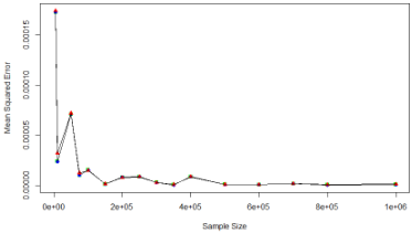
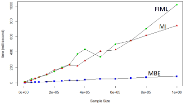
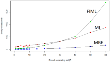
) The first experiment measures the mean squared errors of the three estimators: MI, ML, MBE, and studies how it varies with increase in sample size, for the problem of recovering mean(X) when |Y | = k = 5. The results of this experiment are plotted in figure 4. We further estimated the average time each procedure took in recovering and plotted time vs sample size in figure 5. Figure 4 shows that all three methods (MBE, MI, FIML) work almost identically so far as the quality of estimate of E(X) is concerned. From figure 5 it is clear that MBE (a non-iterative procedure) takes less time in computing E(X) as compared to MI and FIML. While all the reported numbers (MSE and time) are averaged over 50 repetitions with different random estimation problems, for a given problem each individual MSE was computed from 500 simulations. In the next experiment we study the efficiency of these procedures as the complexity of the model increases. In MAR models, complexity of recoverability depends on the size of the separating set Y that d-separates X fromRx (and on the size of the dataset). This experiment was conducted by fixing sample size to 100,000. We observe in Figure 6 that as the separating set becomes larger, the time taken to recover estimates also increases. Note that in this case the time gain pertains to computing parameters of one partially observed variable X. Clearly, in a real world dataset with several partially observed variables, the time savings offered by MBE will be substantial.

Missing Not At Random: The goal here is to evaluate the

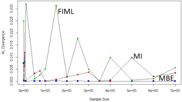
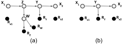
effectiveness of algorithm 1 using data generated by the self masking model in 3. βwy and βzy are not recoverable by lemma 2; hence Z and W cannot be used for recovering var(Y ). However, βx1y is recoverable. We can create a latent projection by treating Z,W,Rz and Rw as latent variables as shown in figure 3 (b). Figure 7 depicts the KL divergence between true and estimated distribution of Y . As expected, FIML and MI behave unpredictably while MBE with minimum KL Divergence behaves ideally.

7 Conclusions

We presented novel graph-based procedures that are noniterative and independent of likelihood function, for recovering parameters in quasi-linear missingness models. We further developed procedures for recovering parameters in self masking models. Finally we showed that given MAR data, our techniques are much faster than state of the art procedures and given MNAR data our techniques can recover parameters where existing techniques fail.

A Proof of theorem 5

B Subroutines used in Algorithm 1

In this subsection we outline the subroutines Recover α and Recove cov invoked by algorithm 1. Recoverability of queries in these subroutines are determined using results in section 4. Note that in this work we only deal with recoverability of statistical parameters. Path coefficients (which are causal parameters) are considered recoverable if (i) they are identifiable and (ii) all factors in the (identified) estimand are recoverable.

Recover αy: Input: G: m-graph in which X1 is a parent of Y and X2 is a child of Y . αy: Path coefficient of edge X1 → Y . Output: αy ∗ if αy is recoverable, NULL otherwise.

• recovered estimands are substituted into the equation above to recover and return the estimand of αy.
• Recover cov: Input: G: m-graph in which X1 is a parent of Y and X2 is a child of Y , αy ∗ : Recovered estimand of αy, the path coefficient of edge X1 → Y . Output: Estimand for cov(X1, Y ) if it is recoverable, NULL otherwise.
• This routine applies lemma 1 on X1 and Y and returns the estimand for recovering cov(X1, Y ) if all variances and path coeffients on the RHS of equation 2 are recoverable.