
Stochastic Anytime Search for Bounding Marginal MAP
Proceedings of the Twenty-Seventh International Joint Conference on Artificial Intelligence. Main track. Pages 5074-5081.
https://doi.org/10.24963/ijcai.2018/704
Keywords
- Heuristic Search and Game Playing: Combinatorial Search and Optimisation
- Heuristic Search and Game Playing: Heuristic Search
- Uncertainty in AI: Graphical Models
- Uncertainty in AI: Bayesian Networks
- Uncertainty in AI: Approximate Probabilistic Inference
Abstract
The Marginal MAP inference task is known to be extremely hard particularly because the evaluation of each complete MAP assignment involves an exact likelihood computation (a combinatorial sum). For this reason, most recent state-of-the-art solvers that focus on computing anytime upper and lower bounds on the optimal value are limited to solving instances with tractable conditioned summation subproblems. In this paper, we develop new search-based bounding schemes for Marginal MAP that produce anytime upper and lower bounds without performing exact likelihood computations. The empirical evaluation demonstrates the effectiveness of our new methods against the current best-performing search-based bounds.
- [Bidyuk et al., 2010] Bozhena Bidyuk, Rina Dechter, and Emma Rollon. Active tuples-based scheme for bounding posterior beliefs. J. Artif. Intell. Res., 39:335-371, 2010.
- [Bonet and Geffner, 2005] Blai Bonet and Hector Geffner. An algorithm better than AO*? In Proceedings of the 20th National Conference on Artificial Intelligence (AAAI), pages 1343-1347, 2005.
- [Bonet and Geffner, 2012] Blai Bonet and Hector Geffner. Action selection for MDPs: Anytime AO* versus UCT. In Proceedings of 26th AAAI Conference on Artificial Intel- ligence (AAAI), pages 1749-1755, 2012.
- [Dechter and Mateescu, 2007] Rina Dechter and Robert Ma- teescu. AND/OR search spaces for graphical models. Arti- ficial Intelligence, 171(2-3):73-106, 2007.
- [Dechter and Rish, 2003] Rina Dechter and Irina Rish. Mini- buckets: A general scheme of approximating inference. Journal of ACM, 50(2):107-153, 2003.
- [Dechter, 2013] Rina Dechter. Reasoning with Probabilistic and Deterministic Graphical Models: Exact Algorithms. Synthesis Lectures on Artificial Intelligence and Machine Learning. Morgan & Claypool Publishers, 2013.
- [Kask and Dechter, 2001] Kalev Kask and Rina Dechter. A general scheme for automatic search heuristics from speci- fication dependencies. Artificial Intelligence, 129(1-2):91- 131, 2001.
- [Lee et al., 2016a] Junkyu Lee, Radu Marinescu, and Rina Dechter. Applying search based probabilistic inference algorithms to probabilistic conformant planning: Prelimi- nary results. In Proceedings of International Symposium on Artificial Intelligence and Mathematics (ISAIM), 2016.
- [Lee et al., 2016b] Junkyu Lee, Radu Marinescu, Rina Dechter, and Alexander Ihler. From exact to anytime so- lutions for marginal MAP. In 30th AAAI Conference on Artificial Intelligence (AAAI), pages 1749-1755, 2016.
- [Liu and Ihler, 2011] Q. Liu and A. Ihler. Bounding the parti- tion function using Hölder's inequality. In Int'l Conference on Machine Learning (ICML), pages 849-856, 2011.
- [Liu et al., 2015] Qiang Liu, John Fisher, and Alexander Ihler. Probabilistic variational bounds for graphical models. In Advances in Neural Information Processing Systems (NIPS) 28, pages 1432-1440, 2015.
- [Lou et al., 2018] Qi Lou, Rina Dechter, and Alexander Ihler. Anytime anyspace AND/OR best-first search for bounding marginal MAP. In AAAI Conference on Artificial Intelli- gence (AAAI), pages 860-867, 2018.
- [Luby et al., 1993] Michael Luby, Alistair Sinclair, and David Zuckerman. Optimal speedup of Las Vegas algo- rithms. Information Processing Letters, 47(4):173-180, 1993.
- [Marinescu et al., 2014] Radu Marinescu, Rina Dechter, and Alexander Ihler. AND/OR search for marginal MAP. In Uncertainty in Artificial Intelligence (UAI), pages 563-572, 2014.
- [Marinescu et al., 2017] Radu Marinescu, Junkyu Lee, Rina Dechter, and Alexander Ihler. Anytime best+depth-first search for bounding marginal MAP. In 31th AAAI Confer- ence on Artificial Intelligence, pages 1749-1755, 2017.
- [Maua and Campos, 2012] Denis Maua and Cassio De Cam- pos. Anytime marginal MAP inference. In International Conference on Machine Learning, pages 1471-1478, 2012.
- [Roth, 1996] Dan Roth. On the hardness of approximate reasoning. Artificial Intelligence, 82(1-2):273-302, 1996.
References were extracted automatically from the PDF and may contain errors.
Full text extracted automatically from the PDF; figures, tables and equations may differ. The PDF is the version of record.
1 Introduction
Probabilistic graphical models provide a powerful framework for reasoning about conditional dependency structures over many variables. Marginal MAP (MMAP) distinguishes between maximization variables (called MAP variables) and summation variables; it is more difficult than either max- or sum- inference tasks alone, primarily because summation and maximization operations do not commute, forcing processing along constrained variable orderings that may have significantly higher induced widths [Dechter, 2013]. This implies larger search spaces (when using search algorithms) or larger messages (when using message-passing schemes). MMAP is NP PP -complete but despite its complexity it is often the appropriate task when there exist hidden variables or uncertain parameters.
Current state-of-the-art schemes focus on solvers that provide not only anytime lower bounds but also anytime upper bounds on the optimal MMAP value. Indeed, the most advanced bounding schemes for MMAP combine best-first search with depth-first search over an AND/OR search graph, and were recently shown to be superior to previous approaches in anytime performance [Marinescu et al., 2017].
However, the major drawback of all existing search-based bounding schemes for MMAP is that they rely on exact conditional likelihood evaluations in order to provide anytime lower bounds. That is, evaluating the probability of any full assignment to the MAP variables amounts to solving exactly a sum-inference subproblem which is known to be PP-complete [Roth, 1996]. For this reason, these methods are only applicable to problem instances where the summation subproblem is tractable, which is not typically the case in many practical applications [Lee et al., 2016a].
In this paper, we present two new search-based bounding schemes for MMAP that compute anytime upper and lower bounds on the optimal MMAP value without performing exact summations. Instead, for each of the MAP solutions found, they use only a lower bound on the corresponding likelihood computation. These schemes also implement different strategies for conducting the exploration of the search space. Specifically, ANYSBFS (anytime stochastic best-first AND/OR search) extends the best-first principle by allowing the expansion of those nodes whose heuristic function deems them less promising in order to uncover a potentially suboptimal solution quickly. ANYLDFS (anytime learning depth-first AND/OR search) smoothly interleaves a greedy depth-first search step aimed at quickly finding a suboptimal solution with a learning step that updates the heuristic node values and directs the search towards a more promising region. Our empirical evaluation on various difficult benchmarks demonstrates the effectiveness of the new schemes compared with some of the current best-performing solvers based on hybrid best+first-search. Finally, we should emphasize that our proposed approach can potentially exploit and improve over any lower bounding algorithm for sum-inference. In this work we illustrate our methodology using a recent weighted minibucket scheme augmented with importance sampling [Liu et al., 2015].
2 Background
A graphical model is a tuple M = 〈X,D, F〉, where X = {Xi : i ∈ V } is a set of variables indexed by set V and D = {Di : i ∈ V } is the set of their finite domains of values. F = {ψα : α ∈ F} is a set of discrete positive real-valued factors defined on subsets of variables, where F ⊆ 2V , and we use α ⊆ V and Xα ⊆ X to indicate the scope of factor ψα, i.e., Xα = var(ψα) = {Xi : i ∈ α}. Specifically, ψα : Ωα → R+, where Ωα is the Cartesian product of the domains {Di : i ∈ α}. The factors scopes yield a primal graph whose vertices are the variables and whose edges connect any two variables that appear in the scope of
(c) Context minimal AND/OR search graph
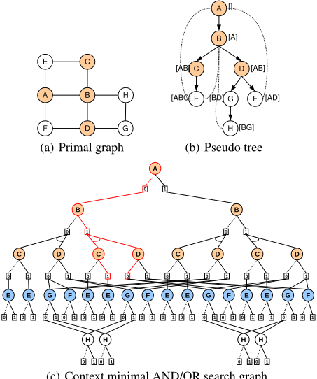
Figure 1: A simple graphical model.
the same factor. The model M defines a factorized probability distribution on X, P(x) = 1Z ∏α∈F ψα(xα). The partition function, Z, normalizes the probability.
Let XM = {X1, ...,Xm} be a subset of X called MAP variables and XS = X \ XM be the complement of XM, called sum variables. The Marginal MAP (MMAP) task seeks an assignment x∗M to variables XM having maximum probability. This requires access to the marginal distribution over XM, which is obtained by summing out variables XS: x∗M = argmaxxM ∑xS ∏α∈F ψα(xα). For numerical stability, the latter is typically solved in log space.
2.1 AND/OR Search Spaces
AND/OR search is guided by a spanning pseudo tree of the graphical model's primal graph (in which any arc of the model not in the tree is a back-arc in the pseudo- tree) and the search space is exponential in the depth of the pseudo tree (rather than in the number of variables). Therefore, mixed inference such as MMAP over a graphical model can be computed by traversing the AND/OR search space [Marinescu et al., 2014].
Definition 1 (pseudo tree). A pseudo tree of an undirected graph G = (V, E) is a directed rooted tree T = (V, E′ ) such that every arc of G not in E′ is a back-arc in T connecting a node in T to one of its ancestors. The arcs in E′ may not all be included in E.
For MMAP we need to restrict the collection of pseudo trees to valid ones. A pseudo tree T is valid for MAP variables XM if T restricted to XM forms a connected start pseudo, a subgraph of pseudo tree T that has the same root as T . Given a graphical model M = 〈X, D, F〉 with primal graph G and valid pseudo tree T of G, the AND/OR search tree ST based on T has alternating levels of OR nodes corresponding to the variables, and AND nodes corresponding to the values of the OR parent's variable, with edge weights extracted from the original functions F (for details see [Dechter and Mateescu, 2007]). Identical sub-problems, identified by their context (the partial instantiation that separates the sub-problem from the rest of the problem graph), can be merged, yielding an AND/OR search graph. Merging all context-mergeable nodes yields the context minimal AND/OR search graph, denoted CT . The size of CT is exponential in the induced width of G along a depth-first traversal of the valid pseudo tree T (also known as the constrained induced width).
Definition 2 (solution subtree). A solution subtree ˆxM of CT relative to the MAP variables XM is a subtree of CT restricted to XM that: (1) contains the root of CT ; (2) if an internal OR node n∈CT is in ˆxM, then n is labeled with a MAP variable and exactly one of its children is in ˆxM; (3) if an internal AND node n∈CT is in ˆxM then all its OR children which denote MAP variables are in ˆxM.
Each node n in CT can be associated with a value v(n); for MAP variables v(n) captures the optimal MMAP value of the conditioned sub-problem rooted at n, while for a sum variable it is the likelihood of the partial assignment denoted by n. It is easy to see that v(n) can be computed recursively based on the values of n's successors, as follows: OR nodes by maximization or summation (for MAP or sum variables, respectively), and AND nodes by multiplication.
Example 1. Figure 1(a) depicts the primal graph of an undirected graphical model representing a distribution over 8 variables, X = A, . . . ,H, with 10 functions defined by the arcs. The highlighted variables XM = {A,B,C,D} denote the MAP variables. Figure 1(b) is a valid pseudo tree (dashed lines denote back-arcs). Figure 1(c) displays the context minimal AND/OR search graph based on the pseudo tree (the contexts are shown next to the pseudo tree nodes). A solution subtree corresponding to the MAP assignment (A=0,B=1,C=1,D=0) is indicated in red.
2.2 Earlier Anytime Search for BoundingMMAP
The two most prominent anytime search methods for bounding MMAP are based on hybrids of best-first and depth-first AND/OR search in order to facilitate the generation of upper bounds (via the best-first component) alongside lower bounds (via the depth-first component) in an anytime fashion [Marinescu et al., 2017]. Specifically, best-first AND/OR search with depth-first lookaheads (LAOBF) traverses the search space in a best-first manner while performing explicit depth-first dives (or lookaheads) below the leaf nodes of the best partial solution tree. Alternating best-first with depth-first AND/OR search (AAOBF) is a parameter-free scheme that interleaves an outer best-first loop with an aggressive depthfirst loop that aims to find improved suboptimal solutions as quickly as possible. Recent extensive empirical evaluations on various difficult benchmarks demonstrated the effectiveness of these schemes compared with previous anytime pure depthfirst and weighted best-first search solvers [Lee et al., 2016b]
Algorithm 1: EXPAND(n) and UPDATE(n)
Input: node n, pseudo tree T , search graph G′T , heuristic function h(·), MAP variables XM = X \ XS 1 Function EXPAND(n): 2 if n is OR node labeled by 〈Xi〉 and Xi ∈ XM then 3 foreach values xi ∈ Di do 4 Create AND child m in G′T labeled by 〈Xi, xi〉 5 if m is terminal then 〈l(m), q(m)〉 ← 〈0, 0〉 6 else 〈l(m), q(m)〉 ← 〈-∞, h(m)〉 7 else if n is AND labeled by 〈Xi, xi〉 and Xi ∈ XM then 8 foreach successors Xj of Xi in T do 9 Create OR child m in G′T labeled by 〈Xj〉 10 if Xj ∈ XS then mark node m as terminal in G′T 11 〈l(m), q(m)〉 ← 〈-∞, h(m)〉 12 Function UPDATE(n): 13 forall the ancestor p of n in G′T , including n do 14 if p is OR node then 15 〈l(p), q(p)〉 ← 〈maxm∈ch(p)(log w(p,m) + l(m)), maxm∈ch(p)(log w(p,m) + q(m))〉 16 m′ ← argmaxm∈ch(p) (logw(p,m) + q(p)) 17 Mark with symbol ⋆ the arc p →m′ 18 else if p is AND node then 19 〈l(p), q(p)〉 ← 〈∑m∈ch(p) l(m), ∑m∈ch(p) q(m)〉as well as with anytime factor set elimination methods [Maua and Campos, 2012].
Weighted Mini-Bucket Heuristics. The effectiveness of the above search algorithms greatly depends on the quality of the upper bound heuristic function that guides the search. Specifically, algorithms AAOBF and LAOBF use a recently developed weighted mini-bucket (WMB) based heuristic [Liu and Ihler, 2011] which can be pre-compiled along the reverse order of the pseudo tree. First, WMB improves the naïve mini-bucket bound [Dechter and Rish, 2003] with Hölder's inequality. For a given variable Xk, the mini-buckets Qkr associated with Xk are assigned a non-negative weight wkr ≥ 0, such that ∑r wkr = 1. Then, each mini-bucket r is eliminated using a powered sum, (∑Xk f(X)1/wkr )wkr . Subsequently, the cost shifting scheme (or reparameterization) is performed across mini-buckets to match the marginal beliefs (or "moments") to further tighten the bound. The single-pass message passing algorithm yields a scheme denoted by WMB-MM(i), where i is called the i-bound and controls the accuracy of the approximation [Dechter and Rish, 2003]. The heuristic can be pre-compiled along a reversed depth-first traversal of a pseudo tree and used to guide the search [Kask and Dechter, 2001; Marinescu et al., 2014].
3 NewAnytime Bounding Schemes
A major limitation of the existing search-based bounding schemes for MMAP is that they rely on exact conditional likelihood computations in order to generate effective lower bounds [Lee et al., 2016b; Marinescu et al., 2017]. Therefore, they are applicable to problem instances with tractable conditioned summations and cannot be used to tackle more difficult problems, which often occur in practice [Lee et al., 2016a]. In this section, we propose two anytime search based schemes that compute upper and lower bounds on the optimal MMAP without performing exact likelihood computations. Our schemes conduct the search over the MAP variables only and propagate upper and lower bounds on the summation parts in the search space to provide improved global upper and lower bounds in an anytime fashion.
3.1 Lower Bounding the Conditioned Summations
The performance of our proposed bounding schemes depends on the quality of the lower bounds on the summation subproblems. In principle, our schemes can potentially exploit and improve over any lower bounding approach for sum-inference, e.g., [Bidyuk et al., 2010]. We elaborate next on two WMB based approaches which we will use. A simple way to compute a lower bound on the partition function Z is to use the WMB scheme with negative instead of positive weights [Liu and Ihler, 2011]. Namely, for a given variable Xk, the mini-buckets Qkr are assigned a negative weight wkr < 0, all except for one which gets a non-negative weight such that ∑ wkr = 1. Then, it can be shown that eliminating all variables (and corresponding mini-buckets) using the power sum operator yields a lower bound ˆ Z on Z.
More recently, [Liu et al., 2015] developed a set of anytime probabilistic bounds that improve directly on the deterministic WMB bounds, combining importance sampling from a WMB-based proposal with concentration inequalities to provide confidence intervals on the true summation value. The method, denoted by WMB-IS(i, δ), was shown to produce a lower bound ˆ Z on Z with at least probability (1 - δ), namely Pr( ˆ Z ≤ Z) ≥ (1-δ), where δ > 0 is known as a confidence value. Since we perform multiple approximations to different conditional summations (corresponding to possible solutions), we use a simple union bound to ensure that our confidence interval on the maximum of our sums is correct. If we perform r conditional sums, we can ensure with confidence δ that:
where ∆(n, δ) is defined in [Liu et al., 2015] eq (8).
3.2 Notations
We denote by G′T the explicated context minimal AND/OR search graph relative to pseudo tree T . In particular, G′T is defined over the MAP variables only with one additional layer of terminal OR nodes labeled by sum variables that root the summation subproblems. A node n ∈ G′T is called a tip (or frontier) node if it has not been expanded yet. An expanded node n ∈ G′T is terminal if it has no successors in G′T . Each node n ∈ G′T maintains two values: q(n) which represents an upper bound provided by the heuristic function at node n, and l(n) which is a lower bound on the optimal solution in the search space below n, respectively. We use U and L to denote the current best global upper and lower bounds on the optimal MMAP value. For node n ∈ G′T , ch(n) denotes its children in G′T , while w(n,m) is the weight labeling the arc n → m in G′T . Algorithm 1 describes the node expansion procedure
Algorithm 2: ANYSBFS
Input: Graphical model M = 〈X, D, F〉, pseudo tree T , heuristic function h(·), XM = X \ XS , probability p, restarts cutoff τ Output: Anytime lower and upper bounds on MMAP value 1 while not TIMEOUT do 2 Create an OR node s labeled by the root of T 3 U = q(s) = h(s), L = l(s) = -∞, G′T = {s}, Tb = {s} 4 while #expansions < τ do 5 Select non-terminal tip node n from G′T \ Tb with probability p, or from Tb with probability (1 - p) 6 EXPAND(n) 7 foreach m ∈ ch(n) do 8 if m is terminal OR node labeled by Xj ∈ XS then 9 l(m) ← max(l(m), LOWERBOUND(m)) 10 UPDATE(n) 11 Let 〈U,L〉 ← 〈q(s),max(L, l(s))〉 and output 〈L, U〉 12 Select new Tb by tracing down ⋆-marked arcs from root s 13 Remove G′T frommemory 14 return 〈L, U〉during search, as well as how the q- and l-values are updated bottom-up based on the corresponding values of their children in the search graph. During the update of q-values, the arc from an OR node n to its best AND child m′ is marked with a ⋆ symbol. These markings are used to compute the current best partial solution subtree Tb in G′T .
Function LOWERBOUND(m) computes a lower bound on the exact summation subproblem rooted at terminal node m in G′T , where m is labeled by a summation variable. For our purpose, we integrated the WMB-IS(i, δ) scheme into LOWERBOUND(m) in order to ensure a true lower bound below m with high probability.
3.3 Anytime Stochastic Best-First Search
Our first bounding scheme is called Anytime Stochastic BestFirst Search (ANYSBFS). The algorithm performs a best-first traversal of the search space that aims at improving the upper bound on the optimal solution value and occasionally expands frontier nodes whose heuristic evaluation function deems them unpromising. Expanding further the subspace below these nodes will eventually uncover suboptimal solutions which in turn yield (anytime) lower bounds on the optimal value. A similar idea was explored by [Bonet and Geffner, 2012] in the context of action selection in MDPs. In contrast to the previous best+depth-first search hybrids AAOBF and LAOBF, algorithm ANYSBFS does not rely on depth-first search traversals to discover improved lower bounds.
ANYSBFS is described by Algorithm 2. Rather than always selecting a tip node fromG′T that is in the current best partial solution tree Tb, ANYSBFS selects with probability p a tip node that does not belong to Tb and thus is in {G′T \ Tb} (line 5). As mentioned earlier, the search is conducted over the MAP variables and therefore the algorithm expands only those nodes that are labeled by MAP variables. Following the expansion of node n, the algorithm updates the q- and l-values of all the ancestors on n in G′T (line 10). Notice that when an
Algorithm 3: ANYLDFS
Input: Graphical model M = 〈X, D, F〉, pseudo tree T , heuristic function h(·), XM = X \ XS Output: Anytime lower and upper bounds on MMAP value 1 Create an OR node s labeled by the root of T 2 U = q(s) = h(s), L = l(s) = -∞, G′T = {s}, Tb = {s} 3 while not TIMEOUT do 4 while tips(Tb) ̸= ∅ OR f(Tb) > L do 5 Select non-terminal tip node n in Tb 6 EXPAND(n) 7 if n is OR node then 8 q(n) ← maxm∈ch(n)(log(w(n,m)) + q(m)) 9 m′ ← argmaxm∈ch(n) (w(n,m) · q(m)) 10 Mark with symbol ⋆ the arc n→m′ 11 Tb ← Tb ∪ {m′ } 12 else if n is AND node then 13 q(n) ← ∑m∈ch(n) q(m) 14 foreach m ∈ ch(n) do 15 if m is terminal OR node labeled by Xi ∈ XS then 16 l(m) ← max(l(m), LOWERBOUND(m)) 17 Tb ← Tb ∪ {ch(n)} 18 forall the nodes m ∈ leaves(Tb) do 19 UPDATE(m) 20 Let 〈U,L〉 ← 〈q(s),max(L, l(s))〉 and output 〈L, U〉 21 Select new Tb by tracing down ⋆-marked arcs from root s 22 return 〈L, U〉AND node n is expanded, if any of its OR children m is labeled by a summation variable (in this case m is a terminal node), then the corresponding node value l(m) is initialized with the lower bound on the conditioned summation subproblem below m computed by function LOWERBOUND(m) (lines 89). During search, the algorithm also keeps track and reports the current best global upper and lower bounds based on the qand l-values of the root node s (line 11). Finally, ANYSBFS continues with the selection of a new best partial solution tree Tb by tracing down the ⋆-marked arcs from the root of G′T or terminates the search if conditions are met.
In order to improve diversification which in turn is likely to yield tighter lower and upper bounds, ANYSBFS employs a restarting strategy. Specifically, the algorithm restarts the search when the number of node expansions exceeds a threshold τ (line 4). The threshold can be fixed, or it can be adaptive following for example a Luby sequence [Luby et al., 1993].
3.4 Anytime Learning Depth-First Search
Our second bounding scheme interleaves a sequence of depthfirst traversals of the search space where a current best partial solution is expanded greedily to a complete solution in order to provide an (anytime) lower bound on the optimal value, with a learning step which consists of a bottom-up revision of the relevant node values in the search space in order to identify the next best partial solution to be explored further as well as to generate an improved upper bound on the optimal solution. Algorithm 3 describes this approach which we call Anytime Learning Depth-First Search (ANYLDFS).
A similar idea was explored by [Bonet and Geffner, 2005] for solving MDPs, and more recently by [Marinescu et al., 2017] for bounding MMAP but in the context of exact summation evaluations. Notice that unlike AAOBF and LAOBF which alternate between best-first and depth-first search in a relatively balanced manner, ANYLDFS uses an aggressive depth-first search exploration of the search space that is aimed at discovering improved lower bounds as quickly as possible.
Specifically, ANYLDFS maintains the global bounds (U and L, respectively) and consists of two main steps. During the first top-down step (lines 4-17), the algorithm expands the current best solution subtree Tb to a solution tree in a greedy depth-first manner, as follows. It selects a tip node n from Tb and expands it by generating its successors. As before, only nodes labeled by MAP variables are expanded further. If n is an OR node then Tb is extended only with n's best AND successor according to its q-value (lines 10-11). Otherwise (it is an AND node), all of n's OR successors are added to Tb. Notice that in the latter case if any of node n's OR successors m is labeled by a summation variable (i.e., m is a terminal node in G′T ) then the corresponding l-value l(m) is initialized with the lower bound on the respective conditioned summation subproblem computed by function LOWERBOUND(m) (lines 14-16). This process stops when Tb becomes a complete solution tree or when it cannot improve over the current global lower bound (line 4). The function f(Tb) is used to compute a heuristic upper bounding estimate on the optimal extension of Tb by summing up the weights on the arcs of Tb with the q-values of the leaf nodes in Tb, respectively.
The second phase is a learning step that updates the node values in G′T bottom-up starting from the leaf nodes of Tb and towards the ancestors of these nodes in G′T (lines 18-19). Following this step, the algorithm uses the q- and l-values of the root node to revise the global upper and lower bounds. Then, it computes the next best partial solution subtree by following the ⋆-marked arcs from the root of G′T and either continues the search or terminates if a time limit is reached.
3.5 Towards Adaptive Bounding Schemes
It is important to notice that unlike the existing best+depth-first search hybrid schemes [Marinescu et al., 2017], algorithms ANYSBFS and ANYLDFS do not mark any of the OR nodes labeled by sum variables as solved when they are first evaluated. This means that the same summation OR node n may be selected and evaluated multiple times during search. Therefore, a possible enhancement applicable to both algorithms is to use an adaptive strategy for sampling, in which each time the same node n is selected for re-evaluation, we increase slightly the time spent by LOWERBOUND(n) for sampling in order to compute a potentially tighter lower bound at the expense of some additional computational overhead.
Unlike their predecessors which rely on exact summation evaluations and thus prove optimality, algorithms ANYSBFS and ANYLDFS equipped with the importance sampling scheme discussed earlier can only produce probabilistic lower bounds that improve with time. However, if function LOWERBOUND(n) implements a bounding scheme that converges to the exact value of the conditioned subproblem below n and if such nodes are marked solved then both algorithms can provide optimality guarantees.
| benchmark | # inst | n | k | w∗ c | w∗ s |
|---|---|---|---|---|---|
| grid | 160 | 144-2500 | 2 | 20-309 | 13-93 |
| pedigree | 110 | 334-1289 | 3-7 | 34-138 | 13-48 |
| promedas | 50 | 453-1849 | 2 | 48-259 | 5-99 |
| planning | 15 | 192-2695 | 3 | 32-446 | 19-207 |
4 Experiments
We evaluate empirically the anytime performance of the proposed algorithms ANYSBFS and ANYLDFS against recent state-of-the-art anytime bounding schemes on benchmark problems generated from standard probabilistic inference networks as well as from planning under uncertainty domains. The competing algorithms, are the earlier AAOBF and LAOBF, respectively, which are the current best-performing best+firstsearch hybrid schemes for providing anytime lower and upper bounds on the optimal MMAP value [Marinescu et al., 2017]. In addition, we also ran LnDFS which is a variant of ANYLDFS explored recently in [Marinescu et al., 2017] that solves the condition summation subproblems exactly. For reference, we also considered UBFS which is a recent bounding scheme for MMAP that is based on best-first search [Lou et al., 2018]. However, unlike our algorithms, UBFS provides anytime upper bounds only. The parameter p that controls the exploration strategy of ANYSBFS was set to 0.5 and its restarts threshold τ followed a standard Luby sequence (1,1,2,1,1,2,4, . . .). All competing algorithms used the same heuristic function WMB-MM(i). We set i = 10 for both the heuristic WMB-MM(i) and the sampling scheme WMB-IS(i), respectively. The time limit was set to 1 hour and we ran all algorithms as memory intensive schemes with a 20GB of RAM limit. We also allowed ANYLDFS and ANYSBFS to perform up to r = 10, 000 calls to the lower bounding scheme for summation within the time limit and we set δ = 0.05 to ensure that they produce true lower bounds with probability at least 95%. Finally, the proposed algorithms also implemented the adaptive strategy described in the previous section and increased the number of samples used by WMB-IS(i) by 25% every time the same summation OR node m is selected for re-evaluation (the initial number of samples was set to 1,000).
Our benchmark set includes 3 standard problem domains from grid networks (grid), genetic linkage analysis (pedigree), and medical diagnosis expert systems (promedas). Since the original problems are pure MAP tasks, we generated 5 synthetic MMAP instances for each pure MAP instance by randomly selecting 10% of the variables as MAP variables. The reason for selecting that many MAP variables was to increase significantly the difficulty of the conditioned summation subproblems. Therefore, we created 160 grid, 110 pedigree, and 50 promedas MMAP instances. In addition, we also considered 15 problem instances derived from probabilistic conformant planning with finite time horizon [Lee et al., 2016a]. These instances correspond to MMAP queries over equivalent dynamic Bayesian network (DBN) encodings of the original planning problems.
time (sec)
time (sec)
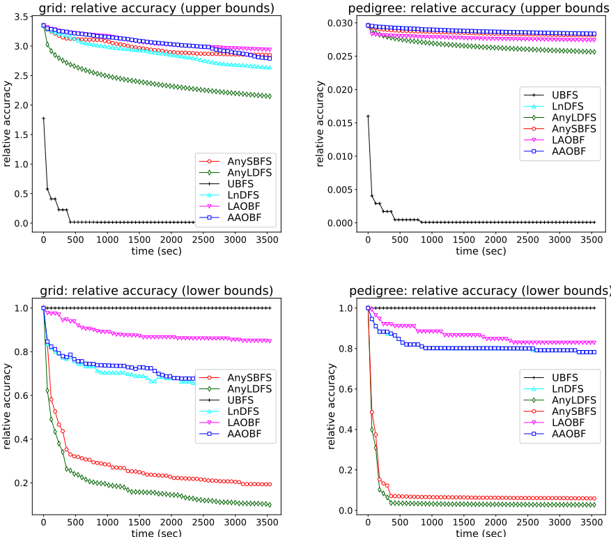
Figure 2: Anytime average relative accuracy with respect to the tightest upper (top) and lower bounds (bottom), respectively.
Table 1 shows the typical ranges of the problem instance parameters where n is the number of variables, k is the domain size, w∗ c is the constrained induced width and w∗ s is the induced width of the conditioned summation subproblem. Note that, this paper illustrates much harder MMAP problem instances compared to previous papers [Lee et al., 2016b; Marinescu et al., 2017].
Responsiveness. The responsiveness characterizes how fast an algorithm can discover non-trivial bounds. For AAOBF, LAOBF, LnDFS, UBFS, ANYSBFS and ANYLDFS, we require them to produce upper bounds other than the initial bounds from the heuristic. Similarly, we require the lower bounds found to be different from the default one -∞. Table 2 shows the number of instances for which each algorithm found non-trivial upper (top) and lower (bottom) bounds within 1 minute, 10 minutes and 1 hour, respectively. The best performance points are highlighted. We can see the ANYSBFS and ANYLDFS significantly outperform AAOBF, LAOBF and LnDFS as they discover non-trivial upper and lower bounds on most of the problem instances, across all time bounds. Most notably, algorithms AAOBF, LAOBF and LnDFS fail to find non-trivial lower bounds on many problem instances, especially on the on the most difficult planning instances because of the sheer difficulty of their conditioned summation subproblems. This is important, because the lower bounds correspond to complete MAP solutions which in turn yield actual plans.
Quality of the Bounds. Table 3 summarizes the winners in terms of finding the tightest upper (top) and lower (bottom) bounds within a given time bound of 1 minute, 10 minutes and 1 hour, respectively. In terms of upper bounds, we can see that UBFS typically finds the tightest bounds, across all reported time bounds. This is because UBFS also explores best-first the subspace associated with the summation subproblem whereas ANYLDFS and ANYSBFS do not. However, in terms of time time lower bounds, we observe that ANYLDFS whose strategy is geared towards finding lower bounds quickly dominates all other algorithms as it discovers the tightest bounds across all domains and time bounds. Algorithms AAOBF and LnDFS produce tighter lower bounds than ANYLDFS only on problem instances where the conditioned summation subproblem is manageable and can be solved exactly.
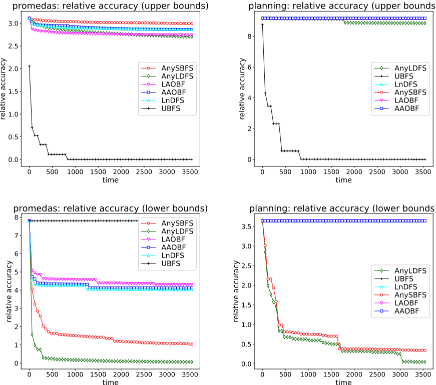
Figure 3: Anytime average relative accuracy with respect to the tightest upper (top) and lower bounds (bottom), respectively.
In Figures 2 and 3 we plot the average relative accuracy with respect to the tightest upper (resp. lower) bounds as a function of time for all four domains and for all competing algorithms. For a given problem instance and algorithm we compute the relative accuracy at time t as |(ut -u∗ )/u∗ )| and |(lt - l∗ )/l∗ |, where ut (resp. lt) is the current upper (resp. lower) bounds and u∗ (resp. l∗ ) is the tightest upper (resp. lower) bound found for that instance. If an algorithm did not find a lower bound at time t then we compute the relative accuracy as |(2 ∗ l- - l∗ )/l∗ |, where l- is the worst lower bound for that particular instance. As before, we see that in terms of upper bounds UBFS is the best performing algorithm, while ANYLDFS dominates in terms of lower bounds. The reduced computational overhead due to bounding the exact summation values allows ANYLDFS to explore a much larger search space which often translates into discovering improved bounds compared to AAOBF/LAOBF/LnDFS.
5 Conclusions
We proposed the first two bounding schemes that compute anytime upper and lower bounds on the optimal MMAP value without evaluating exactly the probability of each MAP assignment generated. The proposed algorithms overcome the most serious limitation of recent search-based bounding schemes that perform the conditional summation computation exactly. Our new algorithms bound the conditional summation using a sampling-based method that generates probabilistic bounds. Our extensive empirical evaluation on various benchmarks demonstrates the effectiveness of the new algorithms compared with existing state-of-the-art bounding schemes. Our approach can accommodate any lower bounding scheme for summation values. Here, we show empirically that exploiting a recent sampling-based probabilistic bounds often yields superior quality bounds on the optimal MMAP.
| algorithm | grid | pedigree | promedas | planning |
|---|---|---|---|---|
| upper bounds (1min/10min/60min) | ||||
| AAOBF LAOBF LnDFS UBFS AnySBFS AnyLDFS | 24/48/61 56/72/87 24/48/64 159/160/160 112/152/159 157/160/160 | 6/20/24 89/91/92 6/20/24 110/110/110 95/103/109 102/109/110 | 14/17/18 44/48/48 14/17/18 50/50/50 49/49/50 50/50/50 | 0/0/0 13/13/13 0/0/0 15/15/15 5/11/14 14/14/15 |
| lower bounds (1min/10min/60min) | ||||
| AAOBF LAOBF LnDFS UBFS AnySBFS AnyLDFS | 24/48/66 2/17/29 24/48/64 0/0/0 160/160/160 160/160/160 | 6/20/24 1/10/19 6/20/24 0/0/0 110/110/110 110/110/110 | 14/17/18 11/15/17 14/17/18 0/0/0 50/50/50 50/50/50 | 0/0/0 0/0/0 0/0/0 0/0/0 15/15/15 15/15/15 |
| algorithm | grid | pedigree | promedas | planning |
|---|---|---|---|---|
| tightest upper bound | ||||
| AAOBF LAOBF LnDFS UBFS AnySBFS AnyLDFS | 0/1/3 0/0/1 1/1/0 158/158/150 0/0/0 2/0/6 | 0/0/0 1/1/2 0/0/0 108/109/107 0/0/0 1/0/1 | 1/0/0 3/0/0 1/0/0 44/50/48 0/0/0 1/0/2 | 0/0/0 1/0/0 0/0/0 14/15/15 0/0/0 0/0/0 |
| tightest lower bound | ||||
| AAOBF LAOBF LnDFS UBFS AnySBFS AnyLDFS | 15/32/40 0/5/5 22/44/51 0/0/0 63/39/35 80/78/74 | 5/16/19 0/1/2 6/14/17 0/0/0 26/24/20 79/66/66 | 9/11/13 0/9/11 13/12/13 0/0/0 1/0/0 36/36/35 | 0/0/0 0/0/0 0/0/0 0/0/0 9/6/3 7/9/12 |
Acknowledgments
This work was supported in part by NSF grants IIS-1526842 and IIS-1254071, and by contracts FA8750-14-C-0011 and W911NF-18-C-0015 under the DARPA PPAML and World Modelers programs. We are grateful to the reviewers for their helpful comments.
@inproceedings{ijcai2018p704,
  title     = {Stochastic Anytime Search for Bounding Marginal MAP},
  author    = {Marinescu, Radu and Dechter, Rina and Ihler, Alexander},
  booktitle = {Proceedings of the Twenty-Seventh International Joint Conference on
               Artificial Intelligence, {IJCAI-18}},
  publisher = {International Joint Conferences on Artificial Intelligence Organization},
  editor    = {Jérôme Lang},
  pages     = {5074--5081},
  year      = {2018},
  month     = {7},
  note      = {Main track},
  doi       = {10.24963/ijcai.2018/704},
  url       = {https://doi.org/10.24963/ijcai.2018/704},
}
TY - CPAPER TI - Stochastic Anytime Search for Bounding Marginal MAP AU - Marinescu, Radu AU - Dechter, Rina AU - Ihler, Alexander T2 - Proceedings of the Twenty-Seventh International Joint Conference on Artificial Intelligence, IJCAI-18 PB - International Joint Conferences on Artificial Intelligence Organization PY - 2018 SP - 5074 EP - 5081 DO - 10.24963/ijcai.2018/704 UR - https://doi.org/10.24963/ijcai.2018/704 ER -Copied
Machine-readable versions of this paper, for tools and AI agents:





