
Implicit Non-linear Similarity Scoring for Recognizing Unseen Classes
Proceedings of the Twenty-Seventh International Joint Conference on Artificial Intelligence. Main track. Pages 4898-4904.
https://doi.org/10.24963/ijcai.2018/680
Keywords
- Computer Vision: Recognition: Detection, Categorization, Indexing, Matching, Retrieval, Semantic Interpretation
- Robotics: Robotics and Vision
- Machine Learning Applications: Networks
Abstract
Recognizing unseen classes is an important task for real-world applications, due to: 1) it is common that some classes in reality have no labeled image exemplar for training; and 2) novel classes emerge rapidly. Recently, to address this task many zero-shot learning (ZSL) approaches have been proposed where explicit linear scores, like inner product score, are employed to measure the similarity between a class and an image. We argue that explicit linear scoring (ELS) seems too weak to capture complicated image-class correspondence. We propose a simple yet effective framework, called Implicit Non-linear Similarity Scoring (ICINESS). In particular, we train a scoring network which uses image and class features as input, fuses them by hidden layers, and outputs the similarity. Based on the universal approximation theorem, it can approximate the true similarity function between images and classes if a proper structure is used in an implicit non-linear way, which is more flexible and powerful. With ICINESS framework, we implement ZSL algorithms by shallow and deep networks, which yield consistently superior results.
- [Akata et al., 2015] Zeynep Akata, Scott E. Reed, Daniel Walter, Honglak Lee, and Bernt Schiele. Evaluation of output embeddings for fine-grained image classification. In CVPR, 2015.
- [Akata et al., 2016] Zeynep Akata, Florent Perronnin, Zaïd Harchaoui, and Cordelia Schmid. Label-embedding for image classification. IEEE Trans. Pattern Anal. Mach. In- tell., 2016.
- [Bishop and others, 2006] Christopher M Bishop et al. Pat- tern recognition and machine learning, volume 1. Springer, New York, 2006.
- [Changpinyo et al., 2016] Soravit Changpinyo, Wei-Lun Chao, Boqing Gong, and Fei Sha. Synthesized classifiers for zero-shot learning. In CVPR, 2016.
- [Chao et al., 2016] Wei-Lun Chao, Soravit Changpinyo, Bo- qing Gong, and Fei Sha. An empirical study and analysis of generalized zero-shot learning for object recognition in the wild. In ECCV, pages 52-68, 2016.
- [Cybenko, 1989] George Cybenko. Approximation by su- perpositions of a sigmoidal function. MCSS, 1989.
- [Donahue et al., 2014] Jeff Donahue, Yangqing Jia, Oriol Vinyals, Judy Hoffman, Ning Zhang, Eric Tzeng, and Trevor Darrell. Decaf: A deep convolutional activation feature for generic visual recognition. In ICML, 2014.
- [Farhadi et al., 2009] Ali Farhadi, Ian Endres, Derek Hoiem, and David A. Forsyth. Describing objects by their at- tributes. In CVPR, 2009.
- [Frome et al., 2013] Andrea Frome, Gregory S. Corrado, Jonathon Shlens, Samy Bengio, Jeffrey Dean, Mar- c'Aurelio Ranzato, and Tomas Mikolov. Devise: A deep visual-semantic embedding model. In NIPS, 2013.
- [Fu et al., 2015] Zhenyong Fu, Tao Xiang, Elyor Kodirov, and Shaogang Gong. Zero-shot object recognition by se- mantic manifold distance. In CVPR, 2015.
- [Guo et al., 2016] Yuchen Guo, Guiguang Ding, Xiaoming Jin, and Jianmin Wang. Transductive zero-shot recognition via shared model space learning. In AAAI, 2016.
- [Guo et al., 2017] Yuchen Guo, Guiguang Ding, Jungong Han, and Yue Gao. Synthesizing samples for zero-shot learning. In IJCAI, pages 1774-1780, 2017. IJCAI
- [He et al., 2016] Kaiming He, Xiangyu Zhang, Shaoqing Ren, and Jian Sun. Deep residual learning for image recog- nition. In CVPR, 2016.
- [Hornik, 1991] Kurt Hornik. Approximation capabilities of multilayer feedforward networks. Neural Networks, 1991.
- [Kodirov et al., 2015] Elyor Kodirov, Tao Xiang, Zhenyong Fu, and Shaogang Gong. Unsupervised domain adaptation for zero-shot learning. In ICCV, 2015.
- [Kodirov et al., 2017] Elyor Kodirov, Tao Xiang, and Shao- gang Gong. Semantic autoencoder for zero-shot learning. In CVPR, 2017. [Krizhevsky et al., 2012] Alex Krizhevsky, Ilya Sutskever, and Geoffrey E. Hinton. Imagenet classification with deep convolutional neural networks. In NIPS, 2012.
- [Lampert et al., 2014] Christoph H. Lampert, Hannes Nick- isch, and Stefan Harmeling. Attribute-based classification for zero-shot visual object categorization. IEEE TPAMI, 2014.
- [Norouzi et al., 2013] Mohammad Norouzi, Tomas Mikolov, Samy Bengio, Yoram Singer, Jonathon Shlens, Andrea Frome, Greg Corrado, and Jeffrey Dean. Zero-shot learn- ing by convex combination of semantic embeddings. CoR- R, abs/1312.5650, 2013.
- [Patterson and Hays, 2012] Genevieve Patterson and James Hays. SUN attribute database: Discovering, annotating, and recognizing scene attributes. In CVPR, 2012.
- [Romera-Paredes and Torr, 2015] Bernardino Romera- Paredes and Philip H. S. Torr. An embarrassingly simple approach to zero-shot learning. In ICML, 2015.
- [Russakovsky et al., 2015] O. Russakovsky, J. Deng, H. Su, J. Krause, S. Satheesh, S. Ma, Z.g Huang, A. Karpathy, A. Khosla, M. S. Bernstein, A. C. Berg, and Fei-Fei Li. Imagenet large scale visual recognition challenge. IJCV, 2015.
- [Sengupta et al., 2016] Nandini Sengupta, Md. Sahidullah, and Goutam Saha. Lung sound classification using cepstral-based statistical features. Comp. in Bio. and Med., 2016.
- [Socher et al., 2013] Richard Socher, Milind Ganjoo, Christopher D. Manning, and Andrew Y. Ng. Zero-shot learning through cross-modal transfer. In NIPS, 2013.
- [Tang et al., 2017] Sheng Tang, Yu Li, Lixi Deng, and Yong- dong Zhang. Object localization based on proposal fusion. IEEE TMM, 2017.
- [Wah et al., 2011] Catherine Wah, Steve Branson, Peter Welinder, Pietro Perona, and Serge Belongie. The Caltech- UCSD Birds-200-2011 Dataset. Technical Report CNS- TR-2011-001, California Institute of Technology, 2011.
- [Xian et al., 2016] Yongqin Xian, Zeynep Akata, Gaurav Sharma, Quynh N. Nguyen, Matthias Hein, and Bern- t Schiele. Latent embeddings for zero-shot classification. In CVPR, 2016.
- [Xian et al., 2017] Yongqin Xian, Christoph H. Lampert, Bernt Schiele, and Zeynep Akata. Zero-shot learning - A comprehensive evaluation of the good, the bad and the ugly. CoRR, abs/1707.00600, 2017.
- [Zhang and Saligrama, 2015] Ziming Zhang and Venkatesh Saligrama. Zero-shot learning via semantic similarity em- bedding. In ICCV, 2015.
- [Zhang and Saligrama, 2016] Ziming Zhang and Venkatesh Saligrama. Zero-shot learning via joint latent similarity embedding. In CVPR, 2016.
- [Zhang et al., 2017] Rui Zhang, Sheng Tang, Yongdong Zhang, Jintao Li, and Shuicheng Yan. Scale-adaptive con- volutions for scene parsing. In ICCV, 2017.
References were extracted automatically from the PDF and may contain errors.
Full text extracted automatically from the PDF; figures, tables and equations may differ. The PDF is the version of record.
1 Introduction
Image classification is an active research topic in artificial intelligence, machine learning and computer vision communities [Bishop and others, 2006]. Recently, the emergence of deep convolutional neural networks has led to tremendous progress for this task and even achieved surpassing-humanlevel performance [He et al., 2016]. But it should be noted the success of current techniques for image classification heavily relies on a large number of labeled training samples for each class. However, collecting a large number of labeled training samples is challenging and expensive in real-world scenarios, like Web image classification, because the number of images for each classes follows a long-tail distribution [Changpinyo et al., 2016] so that many classes have limited, or even no labeled exemplar. In addition, many new concepts emerge every day and it is difficult to collect labeled data for them. In these cases, the recognition model has to recognize classes which are unseen before. Therefore, how to train image recognition models that is capable of generalizing well for unseen classes, i.e., zero-shot learning, has recently become a hot research topic and is an open issue [Xian et al., 2017].
∗This work was supported by the National Natural Science Foundation of China (No. 61571269, 61701273), and the Project Funded by China Postdoctoral Science Foundation (No. 2017M610897). Corresponding authors: Guiguang Ding and Bin Wang.
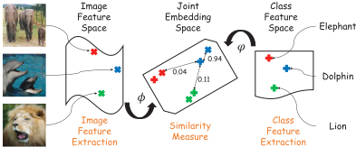
The basic idea of ZSL is to learn a function to measure the correspondence/similarity between an image and a class using seen classes which have sufficient labeled images, and then transfer the similarity function to unseen ones. If an image is very similar to a class, it is likely to belong to this class. We summarize the framework in Figure 1. Each image is represented by a feature vector (image feature extraction), like deep feature [Donahue et al., 2014]. Each class is also given a feature vector (class feature extraction), like the word2vec output using the class name as input or the class attributes [Lampert et al., 2014]. Then the key step is to construct an image feature projection function φ and a text feature projection function ϕ to map them into a joint embedding space such that the similarity between them can be directly measured. The joint embedding space can be the image feature space [Guo et al., 2017], the class feature space [Socher et al., 2013], or a new latent space [Akata et al., 2016]. After the joint embedding step, the similarity between an image and a class can be measured directly in this space, where the explicit linear scoring is widely adopted, for example, inner product similarity [Romera-Paredes and Torr, 2015; Zhang and Saligrama, 2016; Xian et al., 2016]. Because the seen classes and unseen classes are related and similar, although different, the function learning on seen classes can work well on unseen classes. In this way, the model is able to recognize unseen classes based on the transferred knowledge.
1.1 Observation and Contribution
As reviewed in the survey [Xian et al., 2017], we have two important observations. Firstly, existing works pay most attention to learn the projection functions φ and ϕ. Secondly, explicit linear scoring is widely used for similarity measure. In fact, the similarity measure plays an important role in ZSL and finding or approximating the true similarity function between images and classes should be an important learning goal. However, it seems similarity measure has not gained adequate attention but a simple linear one is utilized for convenience. For example, the similarity function in many ZSL approaches [Frome et al., 2013; Norouzi et al., 2013; Socher et al., 2013; Akata et al., 2015; Kodirov et al., 2015; Romera-Paredes and Torr, 2015; Zhang and Saligrama, 2015; Akata et al., 2016; Xian et al., 2016] can be summarized as:
where x and y denote an image and a class, f(x, y) is the similarity function, φ and ϕ are the image-specific and classspecific embedding functions, and W is the linear compatibility parameters. Different approaches may have different choices for these functions. We need to point out although one may utilize non-linear functions for φ and ϕ, these functions can be regarded as the feature extraction functions so that generally f is still linear similarity with explicit scoring.
The simpleness of explicit linear scoring makes it easy to optimize. However, the true similarity function between images and classes is intuitively more than a linear one. Different datasets and scenarios may also have different functions. So explicitly defining a linear similarity function by human knowledge is sometimes not the best choice. On the other hand, using implicit non-linear similarity scoring seems more reasonable and practical. Motivated by this idea, we propose a ICINESS framework for ZSL. In particular, as stated by the universal approximation theorem, a feed-forward network with a single hidden layer containing a finite number of neurons can approximate continuous functions on compact subsets of Rn under mild assumptions on the activation function. Inspired by it, we adopt a neural network to approximate the true similarity function F(x, y). The network uses image and class features as input and output a similarity score directly. In this way, we do not need to specify the definition of f and let the network learn it automatically. In addition, it can learn non-linear similarity function. Obviously, ICINESS is more flexible and powerful than the explicit linear scoring in Eq. (1), which can better approximate the true function F. Moreover, based on ICINESS, it is easy to implement shallow or deep networks to make fully use of the advantages of neural network. We make the following contributions:
1. Different from the explicit linear similarity scoring in many ZSL approaches, we propose a novel implicit nonlinear similarity scoring (ICINESS) for ZSL. Based on the universal approximation theorem, we use a neural network to implicitly approximate the non-linear similarity between images and classes, which can be more powerful and flexible.
2. Based on ICINESS, we implement shallow and deep networks. In practice, many existing ZSL approaches can be regarded as a special linear case of ICINESS but our work can deal with more complicated non-linear similarity functions.
- We conduct extensive experiments on several benchmark datasets. The experimental results demonstrate consistent accuracy improvement over existing approaches for (generalized) ZSL, which validates the effectiveness of ICINESS.
2 Preliminary and RelatedWork
2.1 Problem and Notation
The problem of ZSL is defined as follows. we have two disjoint class sets C s = {cs1 , ..., csks } and C u = {cu1 , ..., cuku } denoting seen classes and unseen classes respectively with C s ∩ C u = ∅, where ks and ku are the number of classes in seen set and unseen set. From the image perspective, a training image set Ds = {xs1 , ..., xsns } is given where each image xsi is associated with one seen class ys i ∈ C s . We uses {xsi , ys i }ns i=1 to learn the similarity function between images and classes. At the test stage, an image xu is given and our goal is to predict its class in the unseen classes yu ∈ C u , which is the standard setting of ZSL. In the generalized ZSL (GZSL) [Xian et al., 2017], an image xt is given. Different from standard ZSL, xt is from C s ∪ C u . To enable similarity measure between images and classes, each class c ∈ C s ∪ C u has a feature vector ac ∈ Rq , which can be class attribute vector [Lampert et al., 2014] or word2vec [Socher et al., 2013].
2.2 RelatedWork
As reviewed before, existing ZSL approaches adopt explicit linear similarity scoring, which can be generally formulated as Eq. (1). The difference is how to choose the embedding functions. Akata et al. [2016], Frome et al. [2013], Akata et al. [2015], Romera-Paredes and Torr [2015], and Kodirov et al. [2017] directly adopted identity function (g(x) = x) for φ and ϕ. The difference is the loss function used to learn W. Socher et al. [2013] utilized a simple two layer neural network for φ, identity function for ϕ and identity matrix for W. Fu et al. [2015] adopted a Markov absorbing chain, while Lampert et al. [2014] employed probabilistic classifier predictions to construct function φ. Zhang and Saligrama [2015] used class independent transformation for φ and sparse coding for ϕ. Norouzi et al. [2013] proposed to use class probability prediction for φ and semantic relatedness for ϕ. In the synthesized classifier approach [Changpinyo et al., 2016], a complicated projection was constructed for ϕ but finally it still used Eq. (1) for similarity measure. In some recent data synthesis approaches [Guo et al., 2017], a reconstruction based algorithm is used to project class features into image feature space for directly linear similarity measurement. In summary, though many ZSL approaches may have linear or non-linear functions for φ and ϕ, they essentially have linear function for similarity measure between images and classes.
3 Implicit Non-linear Similarity Scoring
3.1 General Framework
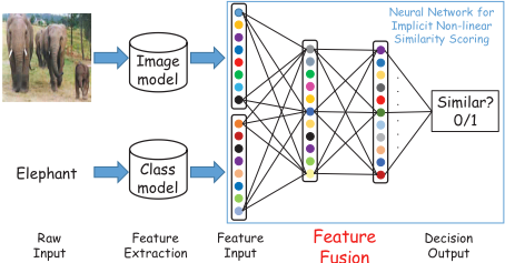
Previous approaches adopt image specific function φ and class specific function ϕ which consider the information from the corresponding side only, and they need to define a specific linear similarity function by human knowledge as in Eq. (1). Due to these limitations, they are not flexible enough and too simple to capture the complicated relationship between images and classes. To address these limitations, a model is expected that takes into account the knowledge from both image and class and captures non-linear imageclass relationship. Since the non-linear similarity is hard to define, the model should approximate it in an implicit way. Fortunately, it is observed that feed-forward neural network is able to approximate non-linear similarity function implicitly. Specifically, based on the universal approximation theorem, a feed-forward network with hidden layers can approximate continuous functions on compact subset of Rn under mild assumptions on the activation function, which has been discussed theoretically [Cybenko, 1989; Hornik, 1991] and applied to a wide range of real-world applications [Krizhevsky et al., 2012; Sengupta et al., 2016]. Inspired by it, we propose a framework ICINESS to implicitly learn the non-linear similarity function for ZSL, as illustrated briefly in Figure 2. In particular, after the feature extraction step for images and classes, we propose to directly fuse image and class features by a few fully connected layers which take both image feature and class feature as input. Then an activation function such as tanh is applied to each unit. The fused features are then connected to an output unit which gives the similarity score for the image-class pair.
It is easy to see the difference from existing approaches. Firstly, suppose the true similarity function is F, existing approaches need to define manually a similarity f explicitly which is likely to be different from F. On the other hand, ICINESS utilizes feed-forward neural network to directly approximate F implicitly without defining f, which is more flexible. Secondly, existing approaches basically adopt linear similarity. On the contrary, ICINESS directly adopts nonlinear activation function, which is capable of capturing nonlinear similarity, which is more powerful. Thirdly, existing approaches process image feature and class feature in a disjoint way such that the relationship between them is not fully explored, while ICINESS adopts a fully connected layer to fuse both features before similarity scoring such that it can better connect image and class features for similarity scoring. Based on these three advantages, ICINESS is able to better explore the cross-modality similarity between image feature and class feature than the explicit linear scoring framework.
3.2 Loss Function and Optimization
Given a training image-class pair {x, y} as input, ICINESS will finally output a similarity score (after a sigmoid function) ˆ s ∈ [0, 1]. The ground truth target is defined as s(x, y) = 1 if image x belongs to class y, or 0 otherwise. One simple way to define the loss function is to use a binary classification (similar/dissimilar) loss, like the cross-entropy loss below:
L(x, y) = -s(x, y) log ˆ s(x, y)-(1-s(x, y)) log(1-ˆ s(x, y)) (2) Compared to the regression based loss function [RomeraParedes and Torr, 2015; Zhang and Saligrama, 2016; Xian et al., 2016; Guo et al., 2016], classification based loss directly optimizes the ZSL goal: judging whether an image-class pair is similar. It is simple to adopt a regression based loss like ‖s - ˆ s‖2 as the loss function. In the experiments, we will show that the classification based loss performs much better.
Fusion
Figure 2: The proposed ICINESS framework. We fuse image and class features in a non-linear way and approximate the image-class similarity by a neural network based universal approximate theorem.
Ranking based loss is also widely used in ZSL. In fact, it is expected not only the similarity to its own class ˆ s(xi, yi) is large, but also larger than any other classes y ̸= yi. Fortunately, it is also very easy to adopt ranking loss in ICINESS. For example, we can adopt triplet loss:
where λ is a positive margin parameter, we use λ = 0.1 here. Based on back-propagation algorithm, it is easy to optimize the network by minimizing the loss function. Specifically, the partial derivative of the cross-entropy loss with respect to ˆ s is:
The partial derivative of the triplet loss with respect to ˆ s is:
where I(z) = 1 if z is true, or 0 otherwise. Since ICINESS adopts basic neural network operations, like convolution layer, fully connected layer, sigmoid, and ReLU, it is easy to back-propagate the gradient of loss functions through the network, especially with well-established neural network tools, like TensorFlow. Then we can use batch-based stochastic gradient descent algorithm to optimize network parameters.
3.3 Implementation
ICINESS is a general framework and flexible. In this paper, we implement a shallow and a deep networks based on it.
Shallow Network. We can view ICINESS as a purely similarity scoring model which takes image feature and class feature as input and output a score. In this case, the "image model" and "class model" in Figure 2 are fixed and we only need the output of them. For example, the image model can be a pre-trained deep convolutional neural network, like ResNet [He et al., 2016] which we use the 2048-dim toplayer pooling units' output as image feature. The class model can be the word2vec tool which gives a 300-dim feature vector using the class name as input, or the class attribute vector [Lampert et al., 2014]. Then with the image feature and class feature as input (the left layer in the blue box in Figure 2), we uses a hidden layer in which each unit is fully connected to both image and class features, followed by an activation function, like tanh. Then all the hidden units are fully connected to the output layer which gives the similarity score ˆ s(x, y). Because the image and class features are given, the network only needs to train hidden fully-connected layers, which can be fast. In our experiment, we find out that this simple shallow network yields state-of-the-art performance.
Deep Network. The shallow network uses pre-trained and fixed image and class models. In fact, we can also train or fine-tune them in ICINESS in an end-to-end manner. In particular, for image model, we adopt ResNet-101 as the base architecture where its top-layer pooling units (we directly use its output as image feature in shallow network) are connected to the hidden fusion layer. As for class feature, we can also use a neural network as class model. In this work, we adopt another fully connected hidden layer to class model. In addition, to relieve the computational burden, we still use the word2vec or class attribute features as raw input of a class. Since the image and class models are fine-tuned, they generate more powerful features, which is able to better fit the data.
For feature fusion, we can use only one hidden layer as briefly shown in Figure 2, which leads to a simple model and is easy to train, or two (or more) hidden layers which is harder to train but can approximate more complicated similarity function. In the experiments, we will show the difference.
3.4 Discussion
Interestingly, we observe that many existing ZSL approaches turn out to be a specific case of ICINESS if proper activation function is utilized. For example, suppose x is the image feature and a is the class feature for y. The similarity function for many linear models [Romera-Paredes and Torr, 2015; Akata et al., 2016; Kodirov et al., 2017] can be written as:
where am is the m-th element in vector a, W∗m is the m-th column in matrix W. Now suppose we have 3 ∗ q hidden units, where the r-th unit is connected to input features with a weight T r ∈ Rd+q where the first d weights correspond to the image feature and the last q weights correspond to the class feature. Then we can set the weights in T as follows:
Then suppose we use square function as the activation function for each hidden unit, and the weights connected to output unit are 1 for the first q hidden units, and -1 for the last 2q units. We can compute the pre-activation output as follows:
| AwA2 | aPY | SUN | CUB | |
|---|---|---|---|---|
| #seen class | 40 | 20 | 645 | 150 |
| #(train) seen sample | 23, 527 | 5, 932 | 10, 320 | 7, 057 |
| #(test) seen sample | 5, 882 | 1, 483 | 2, 580 | 1, 764 |
| #unseen class | 10 | 12 | 72 | 50 |
| #unseen sample | 7, 913 | 7, 924 | 1, 440 | 2, 967 |
| #class attributes | 85 | 64 | 102 | 312 |
which indicates the output of the network is equivalent to linear similarity score. In fact, if the projections φ and ϕ are linear [Zhang and Saligrama, 2015; Norouzi et al., 2013], i.e., φ(x) = xP and ϕ(a) = aR, we can define Wnet = PWR′ and define a network by Eq. (8) using Wnet. This network is equivalent to the original similarity function. For which adopt non-linear projections [Socher et al., 2013; Changpinyo et al., 2016], we can also regard their transformation functions as a feature preprocessing step for ICINESS which is analogous to the deep implementation of ICINESS.
4 Experiment
4.1 Experiment Setting
Following [Xian et al., 2017], we adopt 4 benchmark datasets for ZSL. The first is Animals with Attributes2 (AwA2) [Xian et al., 2017] with 40 seen classes and 10 unseen classes. The second is aPascal-aYahoo (aPY) [Farhadi et al., 2009] with 20 seen classes and 12 unseen classes. The third is SUN [Patterson and Hays, 2012] scene recognition dataset with 645 seen classes and 72 unseen classes. The last is CUB [Wah et al., 2011] bird recognition dataset with 150 seen classes and 50 unseen classes. For each image, we use the 2, 048-dimensional output of the pre-trained ResNet-101 as image feature considering its efficacy [Tang et al., 2017; Zhang et al., 2017]. For each class, the attribute vector from each dataset is used as the class feature. The seen-unseen split is from Xian et al. [2017]. The statistics are in Table 1.
We consider two tasks. The first is standard ZSL, where a test sample is from C u and the goal is to assign a label c ∈ C u to the test sample. For ICINESS, the prediction is given by
where ˆ s(x, c) is the similarity score given by ICINESS. In this case, the performance is evaluated by the average perclass top-1 accuracy [Xian et al., 2017] defined as follows:
where C = C u . We use all samples from the seen classes, including both train and test in Table 1, to train the network.
The second task is generalized ZSL (GZSL) where a test sample may come from both C u and C s and the goal is to assign a label c ∈ C s ∪ C u to the test sample. Because the model is likely to assign larger values to seen classes [Chao et al., 2016], we slightly modify the prediction as follows:
where we simply use γ = 0.1 in this paper. In GZSL, the test data contains two parts. One is the unseen samples and the other is the test seen samples (the fourth row in Table 1). We only use the train seen samples (the third row in Table 1) as the training set. The harmonic mean of the accuracies on seen classes and unseen classes is used as evaluation metric:
4.2 Implementation Details
To alleviate the difference between image feature's scale and class feature's scale, all features are all normalized to have unit length before feed into the network. For feature fusion, 512 hidden units are used for each hidden layer. For the deep implementation, we use ResNet-101 as the backbone for image model, which is pre-trained on ImageNet [Russakovsky et al., 2015]. For each class, we use the attribute vector as input and adopt an one-hidden-layer network as the class model which has 512 hidden units and 128 output units with tanh as the activation function. In fact, because the manually defined attribute vector is itself a good class feature, we also consider to directly use the attributes as the input to the fusion network.
We implement the network in TensorFlow framework. Mini-batch based stochastic gradient descent is used to optimize network parameters with initial learning rate 0.01 and decrease it to 0.001 after 75k batches. The training stops after 100k batches. We use 128 image-class pair in each batch. In particular, a positive pair is given by an image and its ground truth class label. A negative pair is an image and a randomly sampled other class. In fact, because each image belongs to only one class, there are much more negative pairs. In this paper, we set the positive:negative ratio to 1 : 3, i.e., for each positive class, we randomly sample 3 negative classes for an image in a batch. Therefore, each batch has 32 images and each image has 1 positive class and 3 negative classes, leading to 128 pairs in each batch. The weight decay is 5e-5 and we use random flip and random rotate for data augmentation.
4.3 Ablation Study
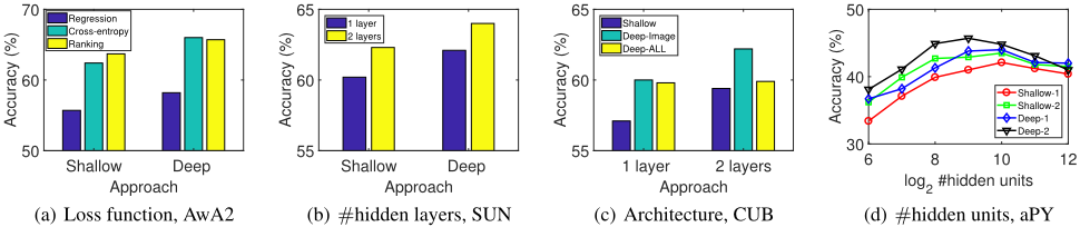
Loss functions. We introduce the cross-entropy classification loss in Eq. (2) and ranking loss in Eq. (3). It is mentioned we can use pre-activation output for regression loss (squared Euclidean loss) like in previous works [Romera-Paredes and Torr, 2015; Zhang and Saligrama, 2016; Guo et al., 2016]. We consider both shallow and deep implementations with one hidden layer. The ZSL accuracy on AwA2 dataset is utilized for evaluation. The comparison is shown in Figure 3(a). Obviously, the classification loss and the ranking loss perform better than the regression loss. In fact, the proposed scoring network attempts to yield large similarity scores for positive pairs and small similarity scores for negative pairs, instead of fitting a particular similarity score, which is more reasonable.
The number of hidden layers. For feature fusion, we can use one hidden layer for simpleness. One hidden layer is able to introduce non-linearity into similarity measure. Also we can adopt more hidden layers to increase the complexity of the model so that it can approximate more complicated similarity function between images and classes. Here we consider the difference between them. We also use shallow and deep implementations and SUN dataset. The results are given in Figure 3(b). It can be observed that two-layer networks achieve higher accuracy than one-layer networks. The superior performance of two-layer networks indicates that imposing more non-linearity is indeed useful for ZSL which is an evidence for the key assumption in this paper that the image-class similarity function is non-linear, which further indicates that the linear functions adopted in previous ZSL works seems too weak to capture the image-class similarity.
The architectures. In the shallow implementation, the image model and class model are fixed while only the fusion layers are tuned. In the deep implementation, we can simultaneously train all parts. In fact, the manually defined class attribute is an effective feature for classes. Therefore, it seems we do not need to train the class model. Instead, we can directly use the attribute vector as the input of fusion layers. Here we investigate the difference between them. In particular, we compare the shallow implementation (Shallow), deep implementation which uses attribute vector for fusion layers directly and only optimizes the image model (Deep-Image), and deep implementation which uses image and attribute attribute vector as raw input for image and class models which are both optimized (Deep-ALL). We use CUB dataset and the results are shown in Figure 3(c). The deep implementations are better than the shallow one. But we observe that DeepALL yields unstable performance while Deep-Image seems more robust. One possible reason is that there are thousands of images and only tens of classes. The class model is likely to overfit the data while the image model is not. Therefore, the fine-tuned image model may better fit the dataset and produce more powerful image feature which leads to better performance than Shallow. However, the overfitted class model may yield worse class feature than the attribute vectors. In the experiments introduced beforehand, we use Deep-Image.
| AwA2 | aPY | SUN | CUB | Average | ||||||
|---|---|---|---|---|---|---|---|---|---|---|
| ACC | H | ACC | H | ACC | H | ACC | H | ACC | H | |
| Norouzi et al. [2013] | 44.5 | 1.0 | 26.9 | 0.0 | 38.8 | 11.6 | 34.3 | 3.1 | 36.13 | 3.93 |
| Changpinyo et al. [2016] | 46.6 | 18.0 | 23.9 | 13.3 | 56.3 | 13.4 | 55.6 | 19.8 | 45.60 | 16.13 |
| Frome et al. [2013] | 59.7 | 27.8 | 39.8 | 9.2 | 56.5 | 20.9 | 52.0 | 32.8 | 52.00 | 22.68 |
| Socher et al. [2013] | 37.9 | 15.9 | 28.0 | 19.0 | 39.9 | 13.3 | 34.6 | 8.7 | 35.10 | 14.23 |
| Lampert et al. [2014] | 46.1 | 0.0 | 33.8 | 9.0 | 39.9 | 7.2 | 40.0 | 3.3 | 39.95 | 4.88 |
| Romera-Paredes and Torr [2015] | 58.6 | 11.0 | 38.3 | 4.6 | 54.5 | 15.8 | 53.9 | 21.0 | 51.33 | 13.10 |
| Xian et al. [2016] | 55.8 | 20.0 | 35.2 | 0.2 | 55.3 | 19.5 | 49.3 | 24.0 | 48.90 | 15.93 |
| Akata et al. [2015] | 61.9 | 14.4 | 32.9 | 6.9 | 53.7 | 19.8 | 53.9 | 33.6 | 50.60 | 18.68 |
| Akata et al. [2016] | 62.5 | 23.9 | 39.7 | 8.7 | 58.1 | 26.3 | 54.9 | 34.4 | 53.80 | 23.33 |
| ICINESS-S | 64.2 | 36.3 | 42.4 | 23.1 | 62.9 | 30.3 | 59.8 | 39.4 | 57.33 | 32.28 |
| ICINESS-D | 67.0 | 41.0 | 46.1 | 25.4 | 65.1 | 32.1 | 62.9 | 41.8 | 60.28 | 35.08 |
The number of hidden units. Now we study the effect the number of units in each hidden layer to the performance. We use aPY, shallow and deep implementations with one or two hidden layers. The ZSL accuracy w.r.t. the number of hidden units is plotted in Figure 3(d). When increasing the number at first, performance gets better because more units lead to more powerful model so that it is capable of approximating more complicated non-linear similarity function. On the other hand, if the model has many hidden units (e.g., 1, 024), further increasing the number may degrade the performance because the model becomes too complicated to train. Using 512 units is a good trade-off between speed and accuracy.
4.4 Benchmark Comparison
We compare ICINESS to the related ZSL approaches on four benchmarks for ZSL and GZSL tasks. In particular, we use the shallow implementation with one hidden layer, denoted as ICINESS-S. It has the same input features as baselines. We also use the Deep-Image with two hidden layers, denoted as ICINESS-D. Both are trained with the cross-entropy loss.
The comparison is summarized in Table 2. ICINESS-S and ICINESS-D both achieve significant improvement over the other baseline approaches for all benchmarks and tasks.
In the experiment, ICINESS-S is almost the simplest implementation of ICINESS. It has the same input features as the baseline approaches, but significantly outperforms them. In particular, the ZSL ACC is improved by 3.53 and the GZSL H by 8.95 in average compared to the best baseline. The baseline approaches all adopt explicit linear scoring, while ICINESS defines the non-linear similarity function in an implicit way. The results clearly demonstrate the superiority of implicit non-linear scoring to explicit linear scoring. As discussed, the image-class similarity is complicated by nature. It is more reasonable to use a non-linear function than a linear one. However, it is quite difficult, if not impossible, to define the function manually. To address this issue, we propose to use a neural network to approximate the function. Based on the universal approximation theorem, neural network is capable of capturing non-linear functions to some extent. Because of this advantage, ICINESS-S achieves much better result.
By using more powerful architectures, ICINESS-D improves average ACC and H by 6.48 and 11.75 respectively compared to the best baseline, which demonstrates its efficacy. By using two hidden layers, ICINESS is able to approximate more complicated non-linear similarity functions. In addition, by fine-tuning the image feature model at the same time, more powerful image features are available. Both issues contribute to the extraordinary performance of ICINESS-D.
5 Conclusion
This paper focuses on zero-shot learning problem. We notice that existing ZSL approaches can be summarized into the same framework, explicit linear similarity scoring which explicitly defines a linear similarity function between images and classes. However, the image-class similarity is complicated by nature so that it seems not reasonable to simply define a linear one. We propose a novel, simple yet effective framework with implicit non-linear similarity scoring (ICINESS) which fuses image feature and class feature by hidden layers to output a similarity score by a network. Based on universal approximation theorem, the network can approximate the true non-linear similarity in an implicit way. We develop shallow and deep versions and we show that many existing ZSL approaches can be regarded as a special case of ICINESS. Experiments on four ZSL benchmarks demonstrate that ICINESS yields better results than the state-of-the-arts.
@inproceedings{ijcai2018p680,
  title     = {Implicit Non-linear Similarity Scoring for Recognizing Unseen Classes},
  author    = {Guo, Yuchen and Ding, Guiguang and Han, Jungong and Zhao, Sicheng and Wang, Bin},
  booktitle = {Proceedings of the Twenty-Seventh International Joint Conference on
               Artificial Intelligence, {IJCAI-18}},
  publisher = {International Joint Conferences on Artificial Intelligence Organization},
  editor    = {Jérôme Lang},
  pages     = {4898--4904},
  year      = {2018},
  month     = {7},
  note      = {Main track},
  doi       = {10.24963/ijcai.2018/680},
  url       = {https://doi.org/10.24963/ijcai.2018/680},
}
TY - CPAPER TI - Implicit Non-linear Similarity Scoring for Recognizing Unseen Classes AU - Guo, Yuchen AU - Ding, Guiguang AU - Han, Jungong AU - Zhao, Sicheng AU - Wang, Bin T2 - Proceedings of the Twenty-Seventh International Joint Conference on Artificial Intelligence, IJCAI-18 PB - International Joint Conferences on Artificial Intelligence Organization PY - 2018 SP - 4898 EP - 4904 DO - 10.24963/ijcai.2018/680 UR - https://doi.org/10.24963/ijcai.2018/680 ER -Copied
Machine-readable versions of this paper, for tools and AI agents:





