
Planning in Factored State and Action Spaces with Learned Binarized Neural Network Transition Models
Proceedings of the Twenty-Seventh International Joint Conference on Artificial Intelligence. Main track. Pages 4815-4821.
https://doi.org/10.24963/ijcai.2018/669
Keywords
- Planning and Scheduling: Other approaches to planning
- Constraints and SAT: Modeling;Formulation
- Planning and Scheduling: Model-Based Reasoning
- Machine Learning: Neural Networks
Abstract
In this paper, we leverage the efficiency of Binarized Neural Networks (BNNs) to learn complex state transition models of planning domains with discretized factored state and action spaces. In order to directly exploit this transition structure for planning, we present two novel compilations of the learned factored planning problem with BNNs based on reductions to Boolean Satisfiability (FD-SAT-Plan) as well as Binary Linear Programming (FD-BLP-Plan). Experimentally, we show the effectiveness of learning complex transition models with BNNs, and test the runtime efficiency of both encodings on the learned factored planning problem. After this initial investigation, we present an incremental constraint generation algorithm based on generalized landmark constraints to improve the planning accuracy of our encodings. Finally, we show how to extend the best performing encoding (FD-BLP-Plan+) beyond goals to handle factored planning problems with rewards.
- [Abío and Stuckey, 2014] Ignasi Abío and Peter J. Stuckey. Encoding linear constraints into sat. In Principles and Practice of Constraint Programming, pages 75-91. Springer Int Publishing, 2014.
- [Amir and Chang, 2008] Eyal Amir and Allen Chang. Learning partially observable deterministic action models. JAIR, 33:349-402, 2008.
- [Audemard and Simon, 2014] Gilles Audemard and Laurent Simon. Lazy Clause Exchange Policy for Parallel SAT Solvers, pages 197-205. Springer Int. Publishing, 2014.
- [Biere et al., 2009] Armin Biere, Marijn Heule, Hans van Maaren, and Toby Walsh, editors. Handbook of Satisfi- ability, volume 185 of Frontiers in Artificial Intelligence and Applications. IOS Press, 2009.
- [Boutilier et al., 1999] Craig Boutilier, Thomas Dean, and Steve Hanks. Decision-theoretic planning: Structural as- sumptions and computational leverage. JAIR, 11(1):1-94, 1999.
- [Collobert et al., 2011] Ronan Collobert, Jason Weston, Leon Bottou, Michael Karlen, Koray Kavukcuoglu, and Pavel Kuksa. Natural language processing (almost) from scratch. JMLR, 12:2493-2537, 2011.
- [Davies et al., 2015] Toby O. Davies, Adrian R. Pearce, Pe- ter J. Stuckey, and Nir Lipovetzky. Sequencing operator counts. In 25th ICAPS, pages 61-69, 2015. IJCAI
- [Davis and Putnam, 1960] Martin Davis and Hilary Putnam. A computing procedure for quantification theory. Journal of the ACM, 7(3):201-215, 1960.
- [Deng et al., 2013] Li Deng, Geoffrey E. Hinton, and Brian Kingsbury. New types of deep neural network learning for speech recognition and related applications: an overview. In IEEE International Conference on Acoustics, Speech and Signal Processing, pages 8599-8603, 2013.
- [Guestrin et al., 2001] Carlos Guestrin, Daphne Koller, and Ronald Parr. Max-norm projections for factored MDPs. In 17th IJCAI, pages 673-680, 2001. IJCAI
- [Helmert, 2006] Malte Helmert. The fast downward plan- ning system. JAIR, 26(1):191-246, 2006.
- [Hubara et al., 2016] Itay Hubara, Matthieu Courbariaux, Daniel Soudry, Ran El-Yaniv, and Yoshua Bengio. Bina- rized neural networks. In 29th NIPS, pages 4107-4115.
- Curran Associates, Inc., 2016.
- [IBM, 2017] IBM. IBM ILOG CPLEX Optimization Studio CPLEX User's Manual, 2017.
- [Ioffe and Szegedy, 2015] Sergey Ioffe and Christian Szegedy. Batch normalization: Accelerating deep net- work training by reducing internal covariate shift. In 32nd ICML, pages 448-456, 2015.
- [Keller and Helmert, 2013] Thomas Keller and Malte Helmert. Trial-based heuristic tree search for finite horizon MDPs. In 23rd ICAPS, pages 135-143, 2013.
- [Kocsis and Szepesvári, 2006] Levente Kocsis and Csaba Szepesvári. Bandit based Monte-Carlo planning. In ECML, pages 282-293, 2006.
- [Krizhevsky et al., 2012] Alex Krizhevsky, Ilya Sutskever, and Geoffrey E. Hinton. Imagenet classification with deep convolutional neural networks. In 25th NIPS, pages 1097- 1105, 2012.
- [Mann and Mannor, 2014] Timothy Mann and Shie Mannor. Scaling up approximate value iteration with options: Bet- ter policies with fewer iterations. In 21st ICML, volume 1, 2014.
- [Nair and Hinton, 2010] Vinod Nair and Geoffrey E. Hinton. Rectified linear units improve restricted boltzmann ma- chines. In 27th ICML, pages 807-814, 2010.
- [Richter and Westphal, 2010] Silvia Richter and Matthias Westphal. The lama planner: Guiding cost-based anytime planning with landmarks. JAIR, 39(1):127-177, 2010.
- [Sanner and Yoon, 2011] Scott Sanner and Sungwook Yoon. International probabilistic planning competition. 2011.
- [Sanner, 2010] Scott Sanner. Relational dynamic influence diagram language (rddl): Language description. 2010.
- [Say et al., 2017] Buser Say, Ga Wu, Yu Qing Zhou, and Scott Sanner. Nonlinear hybrid planning with deep net learned transition models and mixed-integer linear pro- gramming. In 26th IJCAI, pages 750-756, 2017. IJCAI
- [Silver et al., 2016] David Silver, Aja Huang, Christopher J. Maddison, Arthur Guez, Laurent Sifre, George van den Driessche, Julian Schrittwieser, Ioannis Antonoglou, Veda Panneershelvam, Marc Lanctot, Sander Dieleman, Do- minik Grewe, John Nham, Nal Kalchbrenner, Ilya Sutskever, Timothy Lillicrap, Madeleine Leach, Koray Kavukcuoglu, Thore Graepel, and Demis Hassabis. Mas- tering the game of go with deep neural networks and tree search. Nature, pages 484-503, 2016.
- [Silver et al., 2017] David Silver, Thomas Hubert, Julian Schrittwieser, Ioannis Antonoglou, Matthew Lai, Arthur Guez, Marc Lanctot, Laurent Sifre, Dharshan Kumaran, Thore Graepel, Timothy Lillicrap, Karen Simonyan, and Demis Hassabis. Mastering chess and shogi by self-play with a general reinforcement learning algorithm. 2017.
- [Sinz, 2005] Carsten Sinz. Towards an Optimal CNF Encod- ing of Boolean Cardinality Constraints, pages 827-831. Springer Berlin Heidelberg, Berlin, Heidelberg, 2005.
- [Yang et al., 2007] Qiang Yang, Kangheng Wu, and Yunfei Jiang. Learning action models from plan examples using weighted max-sat. AIJ, 171(2):107-143, 2007.
References were extracted automatically from the PDF and may contain errors.
Full text extracted automatically from the PDF; figures, tables and equations may differ. The PDF is the version of record.
1 Introduction
Deep neural networks have significantly improved the ability of autonomous systems to perform complex tasks, such as image recognition [Krizhevsky et al., 2012], speech recognition [Deng et al., 2013] and natural language processing [Collobert et al., 2011], and can outperform humans and humandesigned super-human systems in complex planning tasks such as Go [Silver et al., 2016] and Chess [Silver et al., 2017].
In the area of learning and online planning, recent work on HD-MILP-Plan [Say et al., 2017] has explored a two-stage framework that (i) learns transitions models from data with ReLU-based deep networks and (ii) plans optimally with respect to the learned transition models using mixed-integer linear programming, but did not provide encodings that are able to learn and plan with discrete state variables. As an alternative to ReLU-based deep networks, Binarized Neural Networks (BNNs) [Hubara et al., 2016] have been introduced with the specific ability to learn compact models over discrete variables, providing a new formalism for transition learning and planning in factored [Boutilier et al., 1999] discrete state and action spaces that we explore in this paper. However planning with these BNN transition models poses two nontrivial questions: (i) What is the most efficient compilation of BNNs for planning in domains with factored state and (concurrent) action spaces? (ii) Given that BNNs may learn incorrect domain models, how can a planner repair BNN compilations to improve their planning accuracy?
To answer question (i), we present two novel compilations of the learned factored planning problem with BNNs based on reductions to Boolean Satisfiability (FD-SAT-Plan) and Binary Linear Programming (FD-BLP-Plan). Over three factored planning domains with multiple size and horizon settings, we test the effectiveness of learning complex state transition models with BNNs, and test the runtime efficiency of both encodings on the learned factored planning problems. While there are methods for learning PDDL models from data [Yang et al., 2007; Amir and Chang, 2008] and excellent PDDL planners [Helmert, 2006; Richter and Westphal, 2010], we remark that BNNs are strictly more expressive than PDDL-based learning paradigms for learning concurrent effects in factored action spaces that may depend on the joint execution of one or more actions. Furthermore, while Monte Carlo Tree Search (MCTS) methods [Kocsis and Szepesv´ari, 2006; Keller and Helmert, 2013] including AlphaGo [Silver et al., 2016] and AlphaGoZero [Silver et al., 2016] could technically plan with a BNN-learned black box model of transition dynamics, unlike this work, they would not be able to exploit the BNN transition structure and they would not be able to provide optimality guarantees with respect to the learned model.
To answer question (ii), we introduce an incremental algorithm based on generalized landmark constraints from the decomposition-based cost-optimal classical planner [Davies et al., 2015], where during online planning we detect and constrain invalid sets of action selections from the decision space of the planners and efficiently improve their planning accuracy. Finally, building on the above answers to (i) and (ii), we extend the best performing encoding to handle factored planning problems with general rewards (FD-BLP-Plan+).
In summary, this work provides the first planner capable of learning complex transition models in domains with mixed (continuous and discrete) factored state and action spaces as BNNs and capable of exploiting their structure in satisfiability (or optimization) encodings for planning purposes. Empirical results demonstrate strong performance in both goaloriented and reward-oriented planning in both the learned and original domains, and provide a new transition learning and planning formalism to the data-driven model-based planning community.
2 Preliminaries
Before we present the SAT and BLP compilation of the learned planning problem, we review the preliminaries motivating this work.
2.1 ProblemDefinition
A deterministic factored planning problem is a tuple Π = 〈S,A,C, T, I,G〉 where S = {Sd , Sc } is a mixed set of state variables with discrete Sd and continuous Sc domains, A = {Ad , Ac } is a mixed set of action variables with discrete Ad and continuous Ac domains, C : S × A → {true, false} is a function that returns true if action a ∈ A and state s ∈ S pair satisfies constraints that represent global constraints on state and action variables, T : S × A → S denotes the stationary transition function between time steps t and t + 1, T(st , at ) = st+1 if c(st , at ) = true for all global constraints c ∈ C, and is undefined otherwise. Finally, I ⊂ C is the initial state and G ⊂ C is the goal state constraints over the set and subset of state variables S, respectively. Given a planning horizon H, a solution (i.e. plan) to Π is a value assignment to action at and state st variables such that T(st , at ) = st+1 and c(st , at ) = true for all global constraints c ∈ C and time steps t ∈ {1, . . . ,H}. The RDDL [Sanner, 2010] formalism is extended to handle goal-specifications and used to describe the problem Π.
2.2 Factored Planning with Deep-Net Learned Transition Models
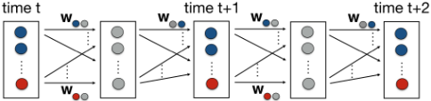
Factored planning with deep-net learned transition models is a two-stage framework for learning and solving nonlinear factored planning problems as first introduced in HD-MILPPlan [Say et al., 2017]. Given samples of state transition data, the first stage of the framework learns the transition function ˜ T using a deep-neural network with Rectified Linear Units (ReLUs) [Nair and Hinton, 2010] and linear activation units. The data is sampled from the RDDL-based domain simulator RDDLsim [Sanner, 2010]. In the second stage, the learned transition function ˜ T is used to construct the factored planning problem ˜Π = 〈S,A,C, ˜ T, I,G〉. That is, the trained deep-neural network with fixed weights is used to predict the state st+1 at time t+1 for free state st and action at variables at time t such that ˜ T(st , at ) = st+1 . As visualized in Figure 1, the learned transition function ˜ T is sequentially chained over horizon t ∈ {1, . . . ,H}, and compiled into a MixedInteger Linear Program yielding the planner HD-MILP-Plan. Since HD-MILP-Plan utilizes only ReLUs and linear activation units in its learned transition models, the state variables s ∈ Sc are restricted to have only continuous domains Sc ⊆ S.
2.3 Binarized Neural Networks
Binarized Neural Networks (BNNs) are neural networks with binary weights and activation functions [Hubara et al., 2016].
During inference, BNNs reduce memory requirements of a system by replacing most arithmetic operations with bit-wise operations. BNN layers are stacked in the following order:
Real or Binary Input Layer: Binary units in all layers, with the exception of the first layer, receive binary input. When the input of the first layer has real-valued domains x ∈ R, m bits of precision can be used for a practical representation such that ˜x = ∑mi=1 2i-1xiwi [Hubara et al., 2016].
Binarization Layer: Given input xj,l of binary unit j ∈ J(l) at layer l ∈ {1, . . . ,L} the deterministic activation function used to compute output yj,l is: yj,l = 1 if xj,l ≥ 0, -1 otherwise, where L denotes the number of layers and J(l) denotes the set of binary units in layer l ∈ {1, . . . , L}.
Batch Normalization Layer: For all layers l ∈ {1, . . . , L}, Batch Normalization [Ioffe and Szegedy, 2015] is a method for transforming the weighted sum of outputs at layer l -1 in ∆j,l = ∑i∈J(l-1) wi,j,l-1yi,l-1 to input xj,l of binary unit j ∈ J(l) at layer l such that: xj,l = ∆j,l-µj,l √σ2 j,l+ϵj,l γj,l+βj,l where parameters wi,j,l-1, µj,l, σ2 j,l , ϵj,l, γj,l and βj,l denote the weight, input mean, input variance, numerical stability constant (i.e., epsilon), input scaling and input bias respectively, where all parameters are computed at training time.
2.4 Boolean Satisfiability Problem
The Boolean Satisfiability Problem (SAT) is the problem of determining whether there exists a value assignment to the variables of a Boolean formula such that the formula evaluates to true (i.e., satisfiable) [Davis and Putnam, 1960]. While the theoretical worst-case complexity of SAT is NPComplete, state-of-art SAT solvers are shown to scale experimentally well for large instances with millions of variables and constraints [Biere et al., 2009].
Boolean Cardinality Constraints
Boolean cardinality constraints describe bounds on the number of Boolean variables that are allowed to be true, and are in the form of AtMostk(x1, . . . , xn) = ∑ni=1 xi ≤ k. An efficient encoding of AtMostk(x1, . . . , xn) in conjunctive normal form (CNF) [Sinz, 2005] is presented below:
Here, si,j are auxiliary Boolean variables implicitly defined in the constraints above. Note that the cardinality constraint ∑ni=1 xi ≤ k is equivalent to ∑ni=1 ¬xi ≥ n - k. For notational clarity, we use AtLeastk(x1, . . . , xn) to denote the cardinality constraint ∑ni=1 xi ≥ k, which is equivalent to AtMostn-k(¬x1, . . . , ¬xn).
2.5 Binary Linear Programming Problem
The Binary Linear Programming (BLP) problem requires finding the optimal value assignment to the variables of a mathematical model with linear constraints, linear objective function, and binary decision variables. Similar to SAT, the theoretical worst-case complexity of BLP is NP-Complete. The state-of-the-art BLP solvers [IBM, 2017] utilize branchand-bound algorithms and can handle cardinality constraints efficiently in the size of its encoding.
2.6 Generalized Landmark Constraints
A generalized landmark constraint is a linear inequality in the form of ∑a∈L(xa ≥ ka) ≥ 1 where L ⊂ A denotes the set of action landmarks and ka denotes counts on actions a ∈ L, that is, the minimum number of times an action must occur in a plan [Davies et al., 2015]. Davies et al. introduced a decomposition-based planner, OpSeq, that incrementally updates generalized landmark constraints to find cost-optimal plans to classical planning problems.
3 SAT Compilation of the Learned Factored Planning Problem
In this section, we show how to reduce the learned factored planning problem ˜Π with BNNs into SAT which we denote as Factored Deep SAT Planner (FD-SAT-Plan).
3.1 Propositional Variables
First, we describe the set of propositional variables used in FD-SAT-Plan. We use three sets of propositional variables: action variables, state variables and BNN binary units, where variables use a bitwise encoding.
- Xia,t denotes if i-th bit of action a ∈ A is executed at time t ∈ {1, . . . ,H}.
- Y i s,t denotes if i-th bit of state s ∈ S is true at time t ∈ {1, . . . , H + 1}.
- Zj,l,t denotes if binary unit j ∈ J(l) at layer l ∈ {1, . . . , L} is activated at time t ∈ {1, . . . ,H}.
3.2 Parameters
Next we define the additional parameters used in FD-SATPlan.
- I is is the initial (i.e., at t = 1) value of the i-th bit of state variable s ∈ S.
- SG is the set of state variables SG ⊆ S specified by the goal constraints G.
- Gis is the goal (i.e., at t = H +1) value of the i-th bit of state variable s ∈ SG.
- In(x, i) is the function that maps the i-th bit of a state or an action variable x ∈ S∪A to the corresponding binary unit in the input layer of the BNN such that In(x, i) = j where j ∈ J(1).
- Out(s, i) is the function that maps the i-th bit of a state variable s ∈ S to the corresponding binary unit in the output layer of the BNN such that Out(s, i) = j where j ∈ J(L).
3.3 The SAT Compilation
Below, we define the SAT encoding of the learned factored planning problem ˜Π with BNNs.
Initial and Goal State Constraints
where clause (1) set the initial and goal values of the state variables at times t = 1 and t = H + 1, respectively.
BNN Constraints
where k in the cardinality constraints is the binary activation threshold computed at training time such that:
for binary unit j ∈ J(l) in layer l ∈ {2, . . . ,L}, where |x| denotes the size of set x, and k′ = |J(l -1)| -k +1 Clauses
(2-3) map the binary units at the input layer of the BNN (i.e., l = 1) to a unique state or action variable, respectively. Similarly, clause (4) maps the binary units at the output layer of the BNN (i.e., l = L) to a unique state variable. Clauses (5-6) encode the binary activation of every unit in the BNN.
Global Constraints
where clause (7) represents domain-dependent global constraints on state and action variables. Some common examples of global constraints c ∈ C such as mutual exclusion on Boolean action variables and one-hot encodings for the output of the BNN (i.e., exactly one Boolean state variable must be true) are respectively encoded below by clauses (8-9):
In general, linear global constraints in the form of ∑i aixi ≤ k, such as bounds on state and action variables, can be encoded in SAT where ai are positive integer coefficients and xi are decision variables with non-negative integer domains [Ab´ıo and Stuckey, 2014].
4 BLP Compilation of the Learned Factored Planning Problem
Given FD-SAT-Plan, we present the BLP compilation of the learned factored planning problem ˜Π with BNNs, which we denote as Factored Deep BLP Planner (FD-BLP-Plan).
4.1 Binary Variables and Parameters
FD-BLP-Plan uses the same set of decision variables and parameters as FD-SAT-Plan.
4.2 The BLP Compilation
FD-BLP-Plan replaces clauses (1-9) with equivalent linear constraints. Clauses (1-4) are replaced by the following equality constraints:
Clause (5) is replaced by the following linear constraint:
for all 1 ≤ t ≤ H, 2 ≤ l ≤ L. Similarly, clause (6) is replaced by the following linear constraint:
for all 1 ≤ t ≤ H, 2 ≤ l ≤ L. Finally, clauses (7-9) are replaced by linear constraints in the form of ∑i aixi ≤ k.
5 Incremental Factored Planning Algorithm for FD-SAT-Plan and FD-BLP-Plan
Now we introduce an incremental algorithm for excluding invalid plans from the search space of FD-SAT-Plan and FDBLP-Plan. Similar to OpSeq [Davies et al., 2015], we update our planners with generalized landmark constraints
where Ln is the set of actions a ∈ A executed at time 1 ≤ t ≤ H at the n-th iteration of the algorithm outlined below.
Algorithm 1 Incremental Factored Planning Algorithm for FD-SAT-Plan and FD-BLP-Plan
- 1: n = 1, planner = FD-SAT-Plan or FD-BLP-Plan
- 2: Ln ← Solve planner.
- 3: if Ln is ∅ or Ln is a plan for Π then
- 4: return Ln
- 5: else planner ←Constraint (17)
- 6: n←n+1, go to line 2.
For a given horizon H, Algorithm 1 iteratively computes a set of actions Ln, or returns infeasibility for the learned factored planning problem ˜Π. If the set of actions Ln is nonempty, we evaluate whether Ln is a valid plan for the original factored planning problem Π (i.e., line 3) either in the actual domain or using a high fidelity domain simulator - in our case RDDLsim. If the set of actions Ln constitutes a plan for Π, Algorithm 1 returns Ln as a plan. Otherwise, the planner is updated with the new set of generalized landmark constraints to exclude Ln and the loop repeats. Since the original action space is discretized and represented upto m bits of precision, Algorithm 1 can be shown to terminate in no more than n = 2|A|×m×H iterations by constructing an inductive proof similar to the termination criteria of OpSeq where either a feasible plan for Π is returned or there does not exist a plan to both ˜Π and Π for the given horizon H.
6 Experimental Results
In this section, we evaluate the effectiveness of factored planning with BNNs. First, we present the benchmark domains used to test the efficiency of our learning and factored planning framework with BNNs. Second, we present the accuracy of BNNs to learn complex state transition models for factored planning problems. Third, we test the efficiency and scalability of planning with FD-SAT-Plan and FD-BLP-Plan on the learned factored planning problems ˜Π across multiple problem sizes and horizon settings. Fourth, we demonstrate the effectiveness of Algorithm 1 to find a plan for the factored planning problemΠ. Finally we test the effectiveness of factored planning with the best performing encoding over the benchmark domains with reward specifications.
6.1 Domain Descriptions
The deterministic RDDL domains used in the experiments, namely Navigation [Sanner and Yoon, 2011], Inventory Control (Inventory) [Mann and Mannor, 2014], and System Administrator (SysAdmin) [Guestrin et al., 2001; Sanner and Yoon, 2011] are described below.
Navigation models an agent in a two-dimensional (m-byn) maze with obstacles where the goal of the agent is to move from the initial location to the goal location at the end of horizon H. The transition function T describes the movement of the agent as a function of the topological relation of its current location to the maze, the moving direction and whether the location the agent tries to move to is an obstacle or not. This domain is a deterministic version of its original from IPPC2011 [Sanner and Yoon, 2011]. Both the action and the state space is Boolean. We report the results on instances with two maze sizes m-by-n and three horizon settings H where m = 3, 4, n = 3, H = 4, 6, 8.
Inventory describes the inventory management control problem with alternating demands for a product over time where the management can order a fixed amount of units to increase the number of units in stock at any given time. The transition function T updates the state based on the change in stock as a function of demand, the current order quantity, and whether an order has been made or not. The action space is Boolean (either order a fixed positive integer amount, or do not order) and the state space is non-negative integer. We report the results on instances with two demand cycle lengths d and three horizon settings H where d = 2, 4 and H = 4, 6, 8.
SysAdmin models the behavior of a computer network P where the administrator can reboot a limited number of computers to keep the number of computers running above a specified safety threshold over time. The transition function T describes the status of a computer which depends on its topological relation to other computers, its age and whether it has been rebooted or not, and the age of the computer which depends on its current age and whether it has been rebooted or not. This domain is a deterministic modified version of its original from IPPC2011 [Sanner and Yoon, 2011]. The action space is Boolean and the state space is a non-negative integer where concurrency between actions are allowed. We report the results on instances with two network sizes |P | and three horizon settings H where |P | = 3, 4 and H = 2, 3, 4.
6.2 Transition Learning Performance
In Table 1, we present test errors for different configurations of the BNNs on each domain instance where the sample data was generated using a simple stochastic exploration policy.
For each instance of a domain, state transition pairs were collected and the data was treated as independent and identically distributed. After random permutation, the data was split into training and test sets with 9:1 ratio. The BNNs were trained on MacBookPro with 2.8 GHz Intel Core i7 16 GB memory using the code available [Hubara et al., 2016]. Overall, Navigation instances required the smallest BNN structures for learning due to their purely Boolean state and action spaces, while both Inventory and SysAdmin instances required larger BNN structures for accurate learning, owing to their non-Boolean state and action spaces.
| Domain | Network Structure | Test Error (%) |
|---|---|---|
| Navigation(3,3) | 12:64:64:9 | 2.12 |
| Navigation(4,3) | 16:80:80:12 | 6.59 |
| Inventory(2) | 7:96:96:5 | 5.51 |
| Inventory(4) | 8:128:128:5 | 4.58 |
| SysAdmin(3) | 12:128:128:9 | 3.73 |
| SysAdmin(4) | 16:96:96:96:12 | 8.99 |
6.3 Planning Performance on the Learned Factored Planning Problems
We compare the effectiveness of using a SAT-based encoding against a BLP-based encoding, namely FD-SAT-Plan and FD-BLP-Plan to find plans for the learned factored planning problem ˜Π. We ran the experiments on MacBookPro with 2.8 GHz Intel Core i7 16GB memory. For FD-SAT-Plan and FDBLP-Plan, we used Glucose [Audemard and Simon, 2014] and CPLEX 12.7.1 [IBM, 2017] solvers respectively, with 30 minutes total time limit per domain instance.
Overall Performance Analysis
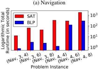
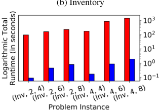
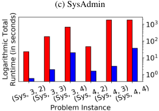
In Figure 2, we present the runtime performance of FD-SATPlan (Red Bar) and FD-BLP-Plan (Blue Bar) over Navigation (Figure 2a), Inventory (Figure 2b) and SysAdmin (Figure 2c) domains. The analysis of the runtime performances across all three domains show that the increase in the size of the underlying BNN structure (as presented in Table 1) significantly increases the computational effort required to find a plan. Similarly for both planners, we observed that increasing the size of the horizon, with the exception of instance (Nav,3,8), increases the cost of computing a plan.
Comparative Performance per Encoding
The pairwise comparison of FD-SAT-Plan and FD-BLP-Plan over all problem settings show a clear dominance of FDBLP-Plan over FD-SAT-Plan in terms of runtime performance. Overall, FD-SAT-Plan computed plans for 15 out of 18 instances while FD-BLP-Plan successfully found plans for all instances. Moreover, with the exception of instances (Nav,4,6) and (Nav,4,8), FD-BLP-Plan found plans for the learned factored planning problems under 20 seconds. On average, FD-BLP-Plan is two orders of magnitude faster than FD-SAT-Plan.
6.4 Planning Performance on the Factored Planning Problems
We test the planning efficiency of the incremental factored planning algorithm using the best performing planner, that is FD-BLP-Plan, for solving the factored planning problem Π. Overall only three instances, namely (Inv,4,8), (Sys,4,3) and (Sys,4,4), required constraint generation to find a plan where the maximum number of constraints required was equal to one. The instances that required the generation of landmark constraints, the runtime performance of FD-BLP-Plan was almost identical to the results presented in Figure 2.
6.5 Planning Performance on the Factored Planning Problems with Reward Specifications
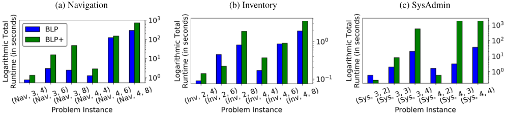
Finally, we extend FD-BLP-Plan to handle domains with reward specifications. Hereby, we extend the definition of the factored planning problem Π to include the reward function Q : S ×A → R such that Π+ = 〈S, A, C, T, I, G, Q〉. Given a planning horizon H, an optimal solution to Π+ is a plan that maximizes the total reward function over all time steps such that ∑Ht=1 Q(st+1 , at ). Similar to HD-MILP-Plan [Say et al., 2017], we assume the knowledge on the reward function Q and add Q as an objective function to our BLP encoding, which we denote as FD-BLP-Plan+.
In Figure 3, we show results for solving the factored planning problems with reward specifications using Algorithm 1. The pairwise comparison of FD-BLP-Plan and FD-BLPPlan+ over all domain instances shows that the additional computational effort required to solve Π+ is minimal, moderate and significant in Inventory, Navigation and SysAdmin domains, respectively. Especially in (Sys,4,3) and (Sys,4,4) instances, FD-BLP-Plan ran out of time at its fifth iteration of Algorithm 1, as the solver could not prove the optimality of the incumbent solution found.
7 Conclusion
In this work, we utilized the efficiency and ability of BNNs to learn complex state transition models of factored planning domains with discretized state and action spaces. We introduced two novel compilations, a SAT (FD-SAT-Plan) and a BLP (FD-BLP-Plan) encoding, that directly exploit the structure of BNNs to plan for the learned factored planning problem, which provide optimality guarantees with respect to the learned model if they successfully terminate. We further introduced an incremental factored planning algorithm based on generalized landmark constraints that improve planning accuracy of both encodings. Finally, we extended the best performing encoding to handle factored planning problems with reward specifications (FD-BLP-Plan+). Empirical results showed we can accurately learn complex state transition models using BNNs and demonstrated strong performance in goal-oriented and reward-oriented planning in both the learned and original domains. In sum, this work provides a novel and effective factored state and action transition learning and planning formalism to the data-driven model-based planning community.
@inproceedings{ijcai2018p669,
  title     = {Planning in Factored State and Action Spaces with Learned Binarized Neural Network Transition Models},
  author    = {Say, Buser and Sanner, Scott},
  booktitle = {Proceedings of the Twenty-Seventh International Joint Conference on
               Artificial Intelligence, {IJCAI-18}},
  publisher = {International Joint Conferences on Artificial Intelligence Organization},
  editor    = {Jérôme Lang},
  pages     = {4815--4821},
  year      = {2018},
  month     = {7},
  note      = {Main track},
  doi       = {10.24963/ijcai.2018/669},
  url       = {https://doi.org/10.24963/ijcai.2018/669},
}
TY - CPAPER TI - Planning in Factored State and Action Spaces with Learned Binarized Neural Network Transition Models AU - Say, Buser AU - Sanner, Scott T2 - Proceedings of the Twenty-Seventh International Joint Conference on Artificial Intelligence, IJCAI-18 PB - International Joint Conferences on Artificial Intelligence Organization PY - 2018 SP - 4815 EP - 4821 DO - 10.24963/ijcai.2018/669 UR - https://doi.org/10.24963/ijcai.2018/669 ER -Copied
Machine-readable versions of this paper, for tools and AI agents:





