Expectation Optimization with Probabilistic Guarantees in POMDPs with Discounted-Sum Objectives

1 Introduction

POMDPs and Discounted-Sum Objectives. Decision making under uncertainty is a fundamental problem in artificial intelligence. Markov decision processes (MDPs) are the de facto model that allows both decision-making choices as well as stochastic behavior [Howard, 1960; Puterman, 2005]. The extension of MDPs with uncertainty about information gives rise to the model of partially-observable Markov decision processes (POMDPs) [Littman, 1996; Papadimitriou and Tsitsiklis, 1987]. POMDPs are used in a wide range of areas, such as planning [Russell and Norvig, 2010], reinforcement learning [Kaelbling et al., 1996], robotics [Kress-Gazit et al., 2009; Kaelbling et al., 1998], to name a few. In decision making under uncertainty, the objective is to optimize a payoff function. A classical and basic payoff function is the discounted-sum payoff, where every transition of the POMDP is assigned a reward, and for an infinite path (that consists of an infinite sequence of transitions) the payoff is the discounted-sum of the rewards of the transitions.

∗This research was supported by the Vienna Science and Technology Fund (WWTF) grant ICT15-003; Austrian Science Fund (FWF): S11407-N23 (RiSE/SHiNE); and an ERC Start Grant (279307: Graph Games).

Expectation Optimization and Drawback. Traditionally, POMDPs with discounted-sum payoff have been studied, where the goal is to obtain policies that optimize the expected payoff. A key drawback of the expectation optimization is that it is not robust with respect to risk measures. For example, a policy σ1 that achieves with probability 1/100 payoff 104 and with the remaining probability payoff 0 has higher expectation than a policy σ2 that achieves with probability 99/100 payoff 100 and with the remaining probability payoff 0. However the second policy is more robust and less risk-prone, and is desirable in many scenarios.

Probability Optimization and Drawback. Due to the drawback of expectation optimization, there has been recent interest to study the optimization of the probability to ensure that the payoff is above a given threshold [Hou et al., 2016]. While this ensures risk-averse policies, it ignores the expectation optimization.

Expectation Optimization with Probabilistic Guarantee. A formulation that retains the advantages of both the above optimization criteria, yet removes the associated drawbacks, is as follows: given a payoff threshold τ and risk bound α, the objective is the expectation maximization w.r.t. to all policies that ensure the payoff is at least τ with probability at least 1 - α. We study this expectation optimization with probabilistic guarantee (EOPG) problem for discounted-sum POMDPs.

Motivating Examples. We present some motivating examples for the EOPG formulation.

• Bad events avoidance. Consider planning under uncertainty (e.g., self-driving cars) where certain events are dangerous (e.g., the distance between two cars less than a specified distance), and it must be ensured that such events happen with low probability. Thus, desirable policies aim to maximize the expected payoff, ensuring the avoidance of bad events with a specified high probability.
• Gambling. In gambling, while the goal is to maximize the expected profit, a desirable risk-averse policy would ensure that the probability loss is less than a given risk.

Thus, the EOPG problem for POMDPs with discounted-sum payoff is an important problem which we consider.

Previous Results. Several related problems have been considered, and two most relevant works are the following:

1. Chance-constrained (CC) problem. In the CC problem, certain bad states of the POMDP must not be reached with some probability threshold. That is, in the CC problem the probabilistic constraint is state-based (some states should be avoided) rather than the execution-based discounted-sum payoff. This problem was considered in [Santana et al., 2016], but only with deterministic policies. As already noted in [Santana et al., 2016], randomized (or mixed) policies are more powerful.
2. Probability 1 bound. The special case of the EOPG problem with α = 0 has been considered in [Chatterjee et al., 2017]. This formulation represents the case with no risk.

Our Contributions. Our main contributions are as follows:

1. Algorithm. We present a randomized algorithm for approximating (up to any given precision) the optimal solution to the EOPG problem. This is the first approach to solve the EOPG problem for discounted-sum POMDPs.
2. Practical approach. We present a practical approach where certain searches of our algorithm are only performed for a time bound. This gives an anytime algorithm which approximates the probabilistic guarantee and then optimizes the expectation.
3. Experimental results. We present experimental results of our algorithm on classical POMDPs.

Due to space constraints, details such as full proofs are deferred to the full version of the paper [Chatterjee et al., 2018].

Related Works. POMDPs with discounted-sum payoff have been widely studied, both for theoretical results [Papadimitriou and Tsitsiklis, 1987; Littman, 1996] as well as practical tools [Kurniawati et al., 2008; Silver and Veness, 2010; Ye et al., 2017]. Traditionally, expectation optimization has been considered, and recent works consider policies that optimize probabilities to ensure discounted-sum payoff above a threshold [Hou et al., 2016]. Several problems related to the EOPG problem have been considered before: (a) for probability threshold 1 for long-run average and stochastic shortest path problem in fully-observable MDPs [Bruy`ere et al., 2014; Randour et al., 2015]; (b) for risk bound 0 for discountedsum payoff for POMDPs [Chatterjee et al., 2017]; and (c) for general probability threshold for long-run average payoff in fully-observable MDPs [Chatterjee et al., 2015b]. The chance constrained-optimization was studied in [Santana et al., 2016]. The general EOPG problem for POMDPs with discountedsum payoff has not been studied before, although development of similar objectives was proposed for perfectly observable MDPs [Defourny et al., 2008]. A related approach for POMDPs is called constrained POMDPs [Undurti and How, 2010; Poupart et al., 2015], where the aim is to maximize the expected payoff ensuring that the expectation of some other quantity is bounded. In contrast, in the EOPG problem the constraint is probabilistic rather than an expectation constraint, and as mentioned before, the probabilistic constraint ensures risk-averseness as compared to the expectation constraint. Thus, the constrained POMDPs and the EOPG problem, though related, consider different optimization criteria.

2 Preliminaries

Throughout this work, we mostly follow standard (PO)MDP notations from [Puterman, 2005; Littman, 1996]. We denote by D(X) the set of all probability distributions on a finite set X, i.e. all functions f : X → [0, 1] s.t. ∑x∈X f(x) = 1.

Definition 1 (POMDPs.) A POMDP is a tuple P = (S,A, δ, r,Z,O, λ) where S is a finite set of states, A is a finite alphabet of actions, δ : S ×A→D(S) is a probabilistic transition function that given a state s and an action a ∈ A gives the probability distribution over the successor states, r : S ×A → R is a reward function, Z is a finite set of observations, O : S → D(Z) is a probabilistic observation function that maps every state to a distribution over observations, and λ ∈ D(S) is the initial belief. We abbreviate δ(s, a)(s′ ) and O(s)(o) by δ(s′ |s, a) and O(o|s), respectively.

Plays & Histories. A play (or an infinite path) in a POMDP is an infinite sequence ρ = s0a1s1a1s2a2 . . . of states and actions s.t. s0 ∈ Supp(λ) and for all i ≥ 0 we have δ(si+1 | si-1, ai) > 0. A finite path (or just path) is a finite prefix of a play ending with a state, i.e. a sequence from (S · A)∗ · S. A history is a finite sequence of actions and observations h = a1o1 . . . ai-1oi ∈ (A · Z)∗ s.t. there is a path w = s0a1s1 . . . aisi with O(oj | sj) > 0 for each 1 ≤ j ≤ i. We write h = H(w) to indicate that history h corresponds to a path w. The length of a path (or history) w, denoted by len(w), is the number of actions in w, and the length of a play ρ is len(ρ) = ∞.

Discounted Payoff. Given a play ρ = s0a1s1a2s2a3 . . . and a discount factor 0 ≤ γ < 1, the finite-horizon discounted payoff of ρ for horizon N is Discγ,N (ρ) = ∑Ni=0 γ i ·r(si, ai+1). The infinite-horizon discounted payoff Discγ of ρ is Discγ(ρ) = ∑∞i=0 γ i · r(si, ai+1).

Policies. A policy (or strategy) is a blueprint for selecting actions based on the past history. Formally, it is a function σ which assigns to a history a probability distribution over the actions, i.e. σ(h)(a) is the probability of selecting action a after observing history h (we abbreviate σ(h)(a) to σ(a | h)). A policy is deterministic if for each history h the distribution σ(· | h) selects a single action with probability 1. For σ deterministic we write σ(h) = a to indicate that σ(a | h) = 1. Beliefs. A belief is a distribution on states (i.e. an element of D(S)) indicating the probability of being in each particular state given the current history. The initial belief λ is given as a part of the POMDP. Then, in each step, when the history observed so far is h, the current belief is bh, an action a ∈ A is played, and an observation o ∈ Z is received, the updated belief bh′ for history h′ = hao can be computed by a standard Bayesian formula [Cassandra, 1998].

Expected Value of a Policy. Given a POMDP P , a policy σ, a horizon N, and a discount factor γ, the expected value of σ from λ is the expected value of the infinite-horizon discounted sum under policy σ when starting in a state sampled from the initial belief of λ of P : eVal (σ) = Eσλ [Discγ,N ].

Risk. A risk level rl (σ, τ, Discγ,N) of a policy σ at threshold τ ∈ R w.r.t. payoff function Discγ,N is the probability that the payoff of a play generated by σ is below τ , i.e.

EOPG Problem. We now define the problem of expectation optimization with probabilistic guarantees (the EOPG problem for short). We first define a finite-horizon variant, and then discuss the infinite-horizon version in Section 3. In EOPG problem, we are given a threshold τ ∈ R, a risk bound α, and a horizon N. A policy σ is a feasible solution of the problem if rl(σ, τ,Discγ,N) ≤ α. The goal of the EOPG problem is to find a feasible solution σ maximizing eVal (σ) among all feasible solutions, provided that feasible solutions exist.

Observable Rewards. We solve the EOPG problem under the assumption that rewards in the POMDP are observable. This means that r(s, a) = r(s′ , a) whenever O(s) = O(s′ ) or if both s and s′ have a positive probability under the initial belief. This is a natural assumption satisfied by many standard benchmarks [Hou et al., 2016; Chatterjee et al., 2015a]. At the end of Section 4 we discuss how could be our results extended to unobservable rewards.

Efficient Algorithms. A standard way of making POMDP planning more efficient is to design an algorithm that is online (i.e., it computes a local approximation of the ε-optimal policy, selecting the best action for the current belief [Ross et al., 2008]) and anytime, i.e. computing better and better approximation of the ε-optimal policy over its runtime, returning a solution together with some guarantee on its quality if forced to terminate early.

3 Relationship to CC-POMDPs

We present our first result showing that an approximate infinitehorizon (IH) EOPG problem can be reduced to a finite-horizon variant. While similar reductions are natural when dealing with discounted payoff, for the EOPG problem the reduction is somewhat subtle due to the presence of the risk constraint. We then show that the EOPG problem can be reduced to chance-constrained POMDPs and solved using the RAO* algorithm [Santana et al., 2016], but we also present several drawbacks of this approach.

Formally, we define the IH-EOPG problem as follows: we are given τ and α as before and in addition, an error term ε. We say that an algorithm ε-solves the IH-EOPG problem if, whenever the problem has a feasible solution (feasibility is defined as before, with Discγ,N replaced by Discγ), the algorithm finds a policy σ s.t. rl (σ, τ - ε, Discγ) ≤ α and Eσλ [Discγ ] ≥ rVal (τ, α) - ε, where

Infinite to Finite Horizon. Let P be a γ-discounted POMDP, τ a payoff threshold, α ∈ [0, 1] a risk bound, and ε > 0 an error term. Let N(ε) be a horizon such that the following holds: γN(ε) · |max{0, rmax}-min{0, rmin}| ≤ (1-γ) · ε2 , where rmax and rmin are the maximal and minimal rewards appearing in P, respectively.

Lemma 1 If there exists a feasible solution of the IH-EOPG problem with threshold τ and risk bound α. Then there exists a policy σ satisfying rl (σ, τ - ε2 , Discγ,N(ε)) ≤ α. Moreover, let σ be an optimal solution to the EOPG problem with the risk bound α, horizon N(ε), and with threshold τ ′ = τ - ε2 . Then σ is an ε-optimal solution to the IH-EOPG problem.

The previous lemma effectively shows that to solve an approximate version of the EOPG problem, it suffices to solve its finite horizon version.

Chance-Constrained POMDPs. In the chance constrained (CC) optimization problem [Santana et al., 2016], we are given a POMDP P, a finite-horizon bound N ∈ N, and a set of constraint-violating states X, which is a subset of the set of states of P. We are also given a risk bound ∆. The goal is to optimize the expected finite-horizon payoff, i.e. the expectation of the following random variable:

The optimization is subject to a constraint that the probability of entering a state from C (so-called execution risk) stays below the risk bound ∆.

From EOPGs to CC-POMDPs. We sketch how the FHEOPG relates to CC-POMDP optimization. In the EOPG problem, the constraint violation occurs when the finite-horizon discounted payoff in step N is smaller than a threshold τ . To formulate this in a CC-POMDP setting, we need to make the constraint violation a property of a state of the POMDP. Hence, we construct a new POMDP P ′ with an extended state space: the states of P ′ are triples of the form ˜ t = (s, i, x), where s is a state of the original POMDP P , 0 ≤ i ≤ N(ε) is a time index, and x ∈ R is a number representing the discounted reward accumulated before reaching the state ˜ t. The remaining components of P ′ are then extended in a natural way from P . By solving the CC-POMDP problem for P ′ , where the set X contains extended states (s, N, x) where x < τ , we obtain a policy in P ′ which can be carried back to P where it forms an optimal solution of the FH-EOPG problem.

Discussion of the CC-POMDP Approach. It follows that we could, in principle, reduce the EOPG problem to CC-POMDP optimization and then solve the latter using the known RAO* algorithm [Santana et al., 2016]. However, there are several issues with this approach.

First, RAO* aims to find an optimal deterministic policy in CC-POMDPs. But as already mentioned in [Santana et al., 2016], the optimal solution to the CC-POMDP (and thus also to EOPG) problem might require randomization, and deterministic policies may have arbitrarily worse expected payoff than randomized ones (it is well-known that randomization might be necessary for optimality in constrained (PO)MDPs, see [Feinberg and Shwartz, 1995; Kim et al., 2011; Sprauel et al., 2014]).

Second, although RAO* converges to an optimal constrained deterministic policy, it does not provide anytime guarantees about the risk of the policy it constructs. RAO* is an AO*-like algorithm that iteratively searches the belief space and in each step computes a greedy policy that is optimal on the already explored fragment of the belief space. During its execution, RAO* works with an under-approximation of a risk taken by the greedy policy: this is because an optimal risk to be taken in belief states that were not yet explored is under-approximated by an admissible heuristic. So if the algorithm is stopped prematurely, the actual risk taken by the current greedy policy can be much larger than indicated by the algorithm. This is illustrated in the following example.

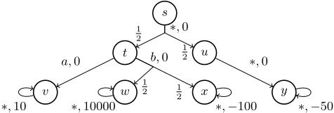
Example 1 Consider the MDP in Figure 1, and consider τ = 1 and α = 23 ; that is, in the chance-constrained reformulation, we seek an optimal policy for which the probability of hitting x and y is at most 23 . Consider the execution of RAO* which explores states s, t, v, w, and x (since the MDP is perfectly observable, we work directly with states) and then is prematurely terminated. (The order in which unexplored nodes are visited is determined by a heuristic, and in general we cannot guarantee that u is explored earlier in RAO*'s execution). At this moment, the risk taken by an optimal policy from u is under-approximated using an admissible heuristic. In case of using a myopic heuristic, as suggested in [Santana et al., 2016], the risk from u is under-approximated by 0. Hence, at this moment the best greedy policy satisfying the risk constraint is the one which plays action b in state t: the risk-estimate of this policy is 14 < 23 (the probability of reaching x). However, any deterministic policy that selects b in state t takes an overall risk 3 4 > 23 .

4 Risk-Aware POMCP

The previous example illustrates the main challenge in designing an online and anytime algorithm for the (finite horizon) EOPG problem: we need to keep upper bounds on the minimal risk achievable in the POMDP. Initially, the upper bound is 1, and to decrease it, we need to discover a sufficiently large probability mass of paths that yield payoff above τ .

We propose an algorithm for the EOPG problem based on the popular POMCP [Silver and Veness, 2010] planning algorithm: the risk-aware POMCP (or RAMCP for short). RAMCP solves the aforementioned challenge by performing, in each decision step, a large number of simulations using the POMCP heuristic to explore promising histories first. The key feature of RAMCP is that it extends POMCP with a new data structure, so called explicit tree, which contains those histories explored during simulations that have payoff above the required threshold τ. The explicit tree allows us to keep track of the upper bound on the risk that needs to be taken

Algorithm 1: RAMCP.

global thr , rbound , n, Tsrch , Texp 1 thr ← τ; rbound ←α; n←N; 2 Tsrch ← Texp ← empty history ϵ 3 initialize ϵ.U = 1 4 while n > 0 do 5 Explore(n) 6 SelectAction() 7 n←n-1 procedure Explore(n) 8 h ← the root of Tsrch; s ← sample from bh 9 while not timeout do Simulate(s, h, n, 0)

from the initial belief. After the simulation phase concludes, RAMCP uses the explicit tree to construct a perfectly observable tree-shaped constrained MDP [Altman, 1999] encoding the EOPG problem on the explored fragment of the history tree of the input POMDP. The optimal distribution on actions is then computed using a linear program for constrained MDP optimization [Altman, 1999]. In the rest of this section, we present details of the algorithm and formally state its properties. In the following, we fix a POMDP P , a horizon N, a threshold τ and a risk bound α.

RAMCP. The main loop of RAMCP is pictured in Algorithm 1. In each decision step, RAMCP performs a search phase followed by action selection followed by playing the selected action (the latter two performed within SelectAction procedure). We describe the three phases separately.

RAMCP: Search Phase. The search phase is shown in Algorithms 1 and 2. We first introduce the data structures the algorithm works with, then the elements of these structures, and finally we sketch how the search phase executes.

Data Structures. In the search phase, RAMCP explores, by performing simulations, the history tree TP of the input POMDP P. Nodes of the tree are the histories of P of length ≤ N. The tree is rooted in the empty history, and for each history h of length at most N - 1, each action a, and observation o, the node h has a child hao. RAMCP works with two data structures, that are both sub-trees of TP : a search tree Tsrch and explicit tree Texp. Intuitively, Tsrch corresponds to the standard POMCP search tree while Texp is a sub-tree of Tsrch containing histories leading to payoff above τ . The term "explicit" stems from the fact that we explicitly compute beliefs and transition probabilities for the nodes in Texp. Initially (before the first search phase), both Tsrch and Texp contain a single node: empty history.

Elements of Data Structures. Each node h of Tsrch has these attributes: for each action a there is h.Va, the average expected payoff obtained from the node h after playing a during past simulations, and h.Na, the number of times action a was selected in node h in past simulations. Next, we have h.N, the number of times the node was visited during past simulations. Each node h of Tsrch also contains a particle-filter approximation of the corresponding belief bh. A node h of the explicit tree has an attribute h.U, the upper bound on the risk from belief bh, and, for each action a, attribute h.Ua, the upper bound on the risk when playing a from belief bh. Also, each node

procedure Simulate(s, h, depth, pay) 1 if depth = 0 then 2 if pay ≥ thr then UpdateTrees(h) 3 return 0 4 if h ̸∈ Tsrch then 5 add h to Tsrch 6 return Rollout(s, h, depth, pay) 7 a ← argmaxa h.Va +K · √ logh.N h.Na 8 sample (s′ , o, r) from (δ(· | s, a),O(· | s′ ), r(s, a)) 9 R← r+γ·Simulate(s′ , hao, depth-1, pay +r) 10 (h.N, h.Na) ← (h.N + 1, h.Na + 1) 11 h.Va ← h.Va + R-h.Va h.Na 12 return R procedure Rollout(s, h, depth, pay) 1 if depth = 0 then 2 if pay ≥ thr then UpdateTrees(h) 3 return 0 4 choose a ∈ A uniformly at random 5 sample (s′ , o, r) from (δ(· | s, a),O(· | s′ ), r(s, a)) 6 return r + γ·Rollout(s′ , hao, depth - 1, pay + r) procedure UpdateTrees(h) 1 hold ← shortest prefix of h not in Texp 2 for g prefix of h and strict extension of hold do 3 add g to Texp 4 let g = ˆ gao; add edge (ˆ g, g) to Texp 5 compute p(ˆ g, g) and rew(ˆ g, g) 6 g ← h; R ← 0 7 h.U ← 0 8 repeat 9 let g = ˆ gao 10 foreach a ∈ A do 11 ˆ g.Ua ← 1 - ∑ o∈Z p(ˆ g, ˆ gao) · (1 - ˆ gao.U ) 12 ˆ g.U ← mina∈A ˆ g.Ua 13 if g ̸∈ Tsrch then 14 add g to Tsrch 15 g.N ← 1; g.Na ← 1; R ← R + rew(ˆ g, g) 16 g.Va ← R 17 g ← ˆ g until g = empty history

of Texp contains an exact representation of the corresponding belief, and each edge (h, hao) of the explicit tree is labelled by numbers p(h, hao) = ∑s,s′∈S bh(s) · δ(s′ | s, a) · O(o | s′ ), i.e. by the probability of observing o when playing action a after history h, and rew(h, hao) = rew(h, a), where rew(h, a) is equal to r(s, a) for any state s with bh(s) > 0 (here we use the facts that rewards are observable).

Execution of Search Phase. Procedures Simulate and Rollout are basically the same as in POMCP-within the search tree we choose actions heuristically (in line 7 of Simulate, the number K is POMCP's exploration constant), outside of it we choose actions uniformly at random. However, whenever a simulation succeeds in surpassing the threshold τ , we add the observed history and all its prefixes to both the explicit and search trees (procedure UpdateTrees). Note that computing p(ˆ g, g) on line 5 entails computing full Bayesian updates on the path from hold to h so as to compute exact beliefs of the corresponding nodes. Risk bounds for the nodes corresponding to prefixes of h are updated accordingly using a standard dynamic programming update (lines 9-12), starting from the newly added leaf whose risk is 0 (as it corresponds to a history after which τ is surpassed). We have the following:

Lemma 2 1. At any point there exists a policy σ such that Pσbhroot (Discγ,N-len(hroot ) < thr ) ≤ hroot .U.

1. As timeout →∞, the probability that hroot .U becomes equal to infσ Pσbhroot (Discγ,N-len(hroot ) < thr) before timeout expires converges to 1.

Proof (sketch). For part (1.) we prove the following stronger statement: Fix any point of algorithm's execution, and let L be the length of hroot (the history at the root of Tsrch and Texp) at this point. Then for any node f of Texp there exists a policy σ s.t. Pσbf (Discγ,len(f)-N < (thr - (Discγ,N(f) - Discγ,N(hroot)) · γ-len(f) )/γ len(f)-L) ≤ f.U. The proof proceeds by a rather straightforward induction. The statement of the lemma then follows by plugging the root of Texp into f.

For part (2.), the crucial observation is that as timeout → ∞, with probability converging to 1 the tree Texp will at some point contain all histories of length N (that have hroot as a prefix) whose payoff is above the required threshold. It can be easily shown that at such a point hroot .U = infσ Pσbhroot (Discγ,N-len(hroot ) < thr), and hroot .U will not change any further. □

RAMCP: Action Selection. The action selection phase is sketched in Algorithm 3. If the current risk bound is 1, there is no real constraint and we select an action maximizing the expected payoff. Otherwise, to compute a distribution on actions to select, we construct and solve a certain constrained MDP.

Constructing Constrained MDP. RAMCP first computes a closure ˆ Texp of Texp. That is, first we set ˆ Texp ← Texp and then for each node h ∈ Texp and each action a such that h has a successor of the form hao ∈ Texp (in such a case, we say that a is allowed in h), the algorithm checks if there exists a successor of the form hao′ that is not in Texp; all such "missing" successors of h under a are added to ˆ Texp. Such a tree ˆ Texp defines a perfectly observable constrained MDPM:

• the states ofMare the nodes of ˆ Texp ;
• for each internal node h of ˆ Texp and each action a allowed in h there is probability p(h, hao) of transitioning from h to hao under a (these probabilities sum up to 1 for each h and a thanks to computing the closure). If h is a leaf of ˆ Texp and len(h) < N, playing any action a in h leads with probability 1 to a new sink state sink (sink has self-loops under all actions).

• Rewards inMare given by the function rew; self-loop on the sink and state-action pairs of the form (h, a) with len(h) = N have reward 0. Transitions from the other leaf nodes h to the sink state have reward maxa h.Va. That is, from nodes that were never explored explicitly (and thus have U-attribute equal to 1) we estimate the optimal payoff by previous POMCP simulations.
• We also have a constraint function C assigning penalties to state-action pairs: C assigns 1/γN-len(hroot ) to pairs (h, a) such that h is a leaf of Texp of length N, and 0 to all other state-action pairs.

Solving MDP M. Using a linear programming formulation of constrained MDPs [Altman, 1999], RAMCP computes a randomized policy π in Mmaximizing Eπ [Discγ] under the constraint Eπ [DiscCγ ] ≥ 1 - rbound, where DiscCγ is a discounted sum of incurred penalties. The distribution π is then the distribution on actions used by π in the first step. An examination of the LP in [Altman, 1999] shows that each solution of the LP yields not only the policy π, but also for each action a allowed in the root, a risk vector da , i.e. an |Z|-dimensional vector such that da (o) = PπM(DiscCγ > 0 | a is played and o is received).

Remark 1 (Conservative risk minimization.) Note that M might have no policy satisfying the penalty constraint. This happens when the U-attribute of the root is greater than rbound. In such a case, the algorithm falls back to a policy that minimizes the risk, which means choosing action a minimizing root.Ua (line 6 of SelectAction). In such a case, all da (o) are set to zero, to enforce that in the following phases the algorithm behaves conservatively (i.e., keep minimizing the risk).

Remark 2 (No feasible solution.) When our algorithm fails to obtain a feasible solution, it "silently" falls back to a riskminimizing policy. This might not be the preferred option for safety-critical applications. However, the algorithm recognizes when it cannot guarantee meeting the original risk-constraintthis happens exactly when at the entry to the SelectAction procedure, the U-attribute in the root of Texp is > rbound. Thus, our algorithm has two desirable properties: (a) it can report that it has not obtained a feasible solution; (b) along with that, it presents a risk-minimizing policy.

Lemma 3 Assume that the original EOPG problem has a feasible solution. For a suitable exploration constant K, as timeout →∞, the distribution dπ converges, with probability 1, to a distribution on actions used in the first step by some optimal solution to the EOPG problem.

Proof (sketch). Assuming the existence of a feasible solution, we show that at the time point in which the condition in Lemma 2 (2.) holds (such an event happens with probability converging to 1), the constrained MDP M has a feasible solution. It then remains to prove that the optimal constrained payoff achievable in M converges to the optimal risk-constrained payoff achievable in P. Since rewards in Mare in correspondence with rewards in Texp, it suffices to

procedure SelectAction() 1 if rbound < 1 ∧ root .U < 1 then 2 M←constrained MDP determined by Texp 3 if root.U ≤ rbound then 4 dπ, {da }a∈A ← solve LP formulation of M 5 else 6 dπ, {da }a∈A ← solve risk-minimizing variant of M 7 a ← sample from dπ 8 else 9 a ← arg maxa root .Va 10 da (o) = 1 for each o 11 PlayAction(a, da)

procedure PlayAction(a, da) 1 play action a and receive observation o and reward R 2 thr ← (thr - R)/γ; rbound ← da (o) 3 h ← root of Tsrch (and Texp) 4 Tsrch ← subtree of Tsrch rooted in hao 5 Texp ← subtree of Texp rooted in hao

show that for each leaf h of Texp with len(h) < N and for each action a, the attribute h.Va converges with probability 1 to the optimal expected payoff for horizon N - len(h) achievable in P after playing action a from belief bh. But since the Va attributes are updated by POMCP simulations, this follows (for a suitable exploration constant) from the properties of POMCP (Theorem 1 in [Silver and Veness, 2010], see also [Kocsis and Szepesv´ari, 2006]). □

RAMCP: Playing an Action. The action-playing phase is shown in Algorithm 3. An action is played in the actual POMDP P and a new observation o and reward R are obtained, and thr and rbound are updated. Then, both the tree data structures are pruned so that the node corresponding to the previous history extended by a, o becomes the new root of the tree. After this, we proceed to the next decision step.

Theorem 1 Assume that an EOPG problem instance with a risk bound α and threshold τ has a feasible solution. As timeout →∞, the probability that RAMCP returns a payoff smaller than τ converges to a number ≤ α. For a suitable exploration constant K, the expected return of a RAMCP execution converges to rVal (τ, α).

Proof (sketch). The proof proceeds by an induction on the length of the horizon N, using Lemma 2 (2.) and Lemma 3. □

RAMCP also provides the following anytime guarantee.

Theorem 2 Let u be the value of the U-attribute of the root of Texp after the end of the first search phase of RAMCP execution. Then the probability that the remaining execution of RAMCP returns a payoff smaller than τ is at most max{u, α}.

Unobservable Rewards. RAMCP could be adapted to work with unobservable rewards, at the cost of more computations. The difference is in the construction of the constraint function C: for unobservable rewards, the same history of observations and actions might encompass both paths that have payoff above the threshold and paths that do not. Hence, we would need to compute the probability of paths corresponding to a given branch that satisfy the threshold condition. This could be achieved by maintaining beliefs over accumulated payoffs.

5 Experiments

We implemented RAMCP on top of the POMCP implementation in AI-Toolbox [AI-Toolbox, 2017] and tested on three sets of benchmarks. The first two are the classical Tiger [Kaelbling et al., 1998] and Hallway [Smith and Simmons, 2004] benchmarks naturally modified to contain a risk taking aspect. In our variant of the Hallway benchmark, we again have a robot navigating a grid maze, oblivious to the exact heading and coordinates but able to sense presence of walls on neighbouring cells. Some cells of the maze are tasks. Whenever a task cell is entered, the robot attempts to perform the task. When doing this, there is a certain probability of a good outcome, after which a positive reward is gained, as well as a chance of a bad outcome, after which a negative penalty is incurred. There are different types of tasks in the maze with various expected rewards and risks of bad outcomes. Once a task is completed, it disappears from the maze. There are also "traps" that probabilistically spin the robot around. As a third benchmark we consider an MDP variant of the Hallway benchmark. Since the Tiger benchmark is small, we present results for the larger benchmarks. Our implementation and the benchmarks are available on-line. 1

We ran the benchmarks with different risk thresholds, starting with risk achieved by unconstrained POMCP and progressively decreasing risk until RAMCP no longer finds a feasible solution. For each α we average outcomes of 1000 executions. In each execution, we used a timeout of 5 seconds in the first decision step and 0.1 seconds for the remaining steps. Intuitively, in the first step the agent is allowed a "pre-processing" phase before it starts its operation, trying to explore as much as possible. Once the agent performs the first action, it aims to select actions as fast as possible. We set the exploration constant to ≈ 2 ·X, where X is the difference between largest and smallest undiscounted payoffs achievable in a given instance.

1 https://git.ist.ac.at/petr.novotny/RAMCP-public

The test configuration was CPU: Intel-i5-3470, 3.20GHz, 4 cores; 8GB RAM; OS: Linux Mint 18 64-bit.

Discussion. In Figure 2, we present the results for: (1.) The Hallway POMDP benchmark (|S| = 67584, |A| = 3, |Z| = 43, γ = 0.95,N = 30, τ = 10); (2.) the perfectly observable version of our Hallway benchmark (|S| = 4512, |A| = 3, |Z| = 1, γ = 0.98,N = 120, τ = 10); and (3.) smaller POMDP instance of the Hallway benchmark (|S| = 7680, |A| = 3,|Z| = 33, γ = 0.8, N = 35, τ = 10). In each figure, the x axis represents the risk bound α. For each α considered we plot the following quantities: average payoff (secondary y axis), empirical risk (the fraction of trials in which RAMCP returned payoff < τ , primary y axis) and stated risk (the average of max{α, U-value of the root of Texp after first search phase}, primary y axis). As expected, the stated risk approximates a lower bound on the empirical risk. Also, as risk bound decreases, the average payoff tends to decrease as well, since the risk bound constraints the agent's behaviour. This trend is somewhat violated in some datapoints: this is because in particular for larger benchmarks, the timeout does not allow for enough exploration so as to converge to a tight approximation of the optimal policy. The main bottleneck is the usage of exact belief updates within the explicit tree. An interesting direction for the future is to replace these updates with a particle-filter approximation (in line with POMCP) and thus improve the speed in exchange for weaker theoretical guarantees. Still, already the current version of RAMCP demonstrates the ability to perform risk vs. expectation trade-off in POMDP planning. Comparison with Deterministic Policies. We also ran experiments related to computation of deterministic policies (by computing, in action selection phase, an optimal deterministic policy in the constrained MDP M, which entails solving a MILP problem). For instance, in benchmark (1.) for α = 0.41 the deterministic policy yields expected payoff 645.017 compared to 1166.8 achieved by randomized policy. In benchmark (3.) with α = 0.3 we have expected payoff 107.49 for deterministic vs. 695.81 for randomized policies.

6 Conclusion

In this work, we studied the expected payoff optimization with probabilistic guarantees in POMDPs. We introduced an online algorithm with anytime risk guarantees for the EOPG problem, implemented this algorithm, and tested it on variants of classical benchmarks. Our experiments show that our algorithm, RAMCP, is able to perform risk-averse planning in POMDPs.