
Path Evaluation and Centralities in Weighted Graphs - An Axiomatic Approach
Proceedings of the Twenty-Seventh International Joint Conference on Artificial Intelligence. Main track. Pages 3856-3862.
https://doi.org/10.24963/ijcai.2018/536
Keywords
- Multidisciplinary Topics and Applications: Social Sciences
- Agent-based and Multi-agent Systems: Economic Paradigms, Auctions and Market-Based Systems
Abstract
We study the problem of extending the classic centrality measures to weighted graphs. Unfortunately, in the existing extensions, paths in the graph are evaluated solely based on their weights, which is a restrictive and undesirable assumption for a variety of settings. Given this, we define a notion of the path evaluation function that assesses a path between two nodes by looking not only on the sum of edge weights, but also on the number of intermediaries. Using an axiomatic approach, we propose three classes of path evaluation functions. Building upon this analysis, we present the first systematic study how classic centrality measures can be extended to weighted graphs while taking into account an arbitrary path evaluation function. As an application, we use the newly-defined measures to identify the most well-linked districts in a sample public transport network.
- [Barrat et al., 2004] Alain Barrat, Marc Barthelemy, Ro- mualdo Pastor-Satorras, and Alessandro Vespignani. The architecture of complex weighted networks. Proceedings of the National Academy of Sciences, 101(11):3747-3752, 2004.
- [Brandes and Erlebach, 2005] Ulrik Brandes and Thomas Erlebach. Network analysis: Methodological foundations. Springer-Verlag, 2005.
- [Brandes, 2001] Ulrik Brandes. A faster algorithm for be- tweenness centrality. Journal of mathematical sociology, 25(2):163-177, 2001.
- [Candeloro et al., 2016] Luca Candeloro, Lara Savini, and Annamaria Conte. A new weighted degree centrality mea- sure: The application in an animal disease epidemic. PloS one, 11(11):e0165781, 2016.
- [Cheng et al., 2015] Yew-Yih Cheng, Roy Ka-Wei Lee, Ee- Peng Lim, and Feida Zhu. Measuring centralities for trans- portation networks beyond structures. In Applications of social media and social network analysis, pages 23-39. Springer, 2015.
- [Costa et al., 2007] L da F Costa, Francisco A Rodrigues, Gonzalo Travieso, and Paulino Ribeiro Villas Boas. Char- acterization of complex networks: A survey of measure- ments. Advances in physics, 56(1):167-242, 2007.
- [Dehaene et al., 2008] Stanislas Dehaene, Véronique Izard, Elizabeth Spelke, and Pierre Pica. Log or linear? distinct intuitions of the number scale in western and amazonian indigene cultures. Science, 320(5880):1217-1220, 2008.
- [Faliszewski et al., 2017] Piotr Faliszewski, Piotr Skowron, Arkadii Slinko, and Nimrod Talmon. Multiwinner voting: A new challenge for social choice theory. Trends in Com- putational Social Choice, page 27, 2017.
- [Freeman, 1979] Linton C. Freeman. Centrality in social networks: Conceptual clarification. Social Networks, 1(3):215-239, 1979.
- [Garg, 2009] Manuj Garg. Axiomatic foundations of central- ity in networks. Available at SSRN 1372441, 2009.
- [Goel and Gruhn, 2008] Asvin Goel and Volker Gruhn. A general vehicle routing problem. European Journal of Op- erational Research, 191(3):650-660, 2008.
- [Grando et al., 2016] Felipe Grando, Diego Noble, and Luis C Lamb. An analysis of centrality measures for com- plex and social networks. In IEEE Global Communica- tions Conference (GLOBECOM), pages 1-6, 2016.
- [Jackson, 2008] Matthew O. Jackson. Social and economic networks, volume 3. Princeton university press, 2008.
- [Koschützki et al., 2005] Dirk Koschützki, Katharina Anna Lehmann, Leon Peeters, Stefan Richter, Dagmar Tenfelde- Podehl, and Oliver Zlotowski. Centrality indices. In Net- work Analysis, volume 3418 of Lecture Notes in Computer Science, pages 16-61. Springer, 2005.
- [Newman, 2001] Mark EJ Newman. Scientific collaboration networks. II. shortest paths, weighted networks, and cen- trality. Physical review E, 64(1):016132, 2001.
- [Opsahl et al., 2010] Tore Opsahl, Filip Agneessens, and John Skvoretz. Node centrality in weighted networks: Generalizing degree and shortest paths. Social networks, 32(3):245-251, 2010.
- [Sabidussi, 1966] Gert Sabidussi. The centrality index of a graph. Psychometrika, 31(4):581-603, 1966.
- [Skibski and Sosnowska, 2018] Oskar Skibski and Jadwiga Sosnowska. Axioms for distance-based centralities. In Proceedings of the 32nd AAAI Conference on Artificial In- telligence (AAAI), pages 1218-1225, 2018.
- [Skibski et al., 2018] Oskar Skibski, Tomasz P. Michalak, and Talal Rahwan. Axiomatic characterization of game- theoretic centrality. Journal of Artificial Intelligence Re- search, 62, 2018.
- [Stai et al., 2017] Eleni Stai, Konstantinos Sotiropoulos, Vasileios Karyotis, and Symeon Papavassiliou. Hyper- bolic embedding for efficient computation of path central- ities and adaptive routing in large-scale complex commod- ity networks. IEEE Transactions on Network Science and Engineering, 4(3):140-153, 2017.
- [Watts and Strogatz, 1998] Duncan J. Watts and Steven H. Strogatz. Collective dynamics of small-world networks. Nature, 393(6684):440-442, 1998.
References were extracted automatically from the PDF and may contain errors.
Full text extracted automatically from the PDF; figures, tables and equations may differ. The PDF is the version of record.
1 Introduction
The centrality analysis is one of the key research lines in network science [Brandes and Erlebach, 2005]. While the standard centralities have been widely used, there is a growing need to extend these concepts to more complex networks [Opsahl et al., 2010; Costa et al., 2007; Grando et al., 2016]. In this paper, we consider such an extension to weighted graphs.
Depending on the application at hand, weights (of edges) can represent various attributes [Barrat et al., 2004]. They can represent a distance, travel time or a cost [Goel and Gruhn, 2008]. On the other hand, they can represent intensity of relation, capacity, or a probability of the fact a given edge exists [Watts and Strogatz, 1998]. In result, a bigger weight can represent either a weaker or a stronger connection. We focus on the former settings, i.e., where a connection is stronger if the weight is smaller.
Most well-known centrality measures are either, directly or indirectly, based on the concept of the distance between nodes in the graph [Kosch¨utzki et al., 2005]. In fact, all three standard centralities proposed by Freeman [1979] are based on the notion of distance: the closeness centrality is defined as the inverse of the sum of distances to other nodes; the betweenness centrality counts how often a given node is on the shortest path between any two nodes; furthermore, the degree centrality, arguably the most popular centrality measure, counts the number of edges of a node-thus, it can be interpreted as the number of nodes at the distance 1. There are also other distance-based centrality measures, e.g. the decay, harmonic, and k-step reach centralities [Jackson, 2008].
In result, the key to extending such centrality measures lays in the definition of a distance in weighted graphs. In unweighted graphs, the distance is simply defined as the size of the shortest path, i.e., its number of edges. But how should we evaluate a path in a weighted graph? Usually, a path is assessed by the sum of weights of its edges and, based on this assumption, many authors proposed their extensions of centrality measures to weighted graphs [Brandes, 2001; Barrat et al., 2004; Newman, 2001]. Nevertheless, this assumption is undesirable in various settings. As argued by [Opsahl et al., 2010], looking solely on the sum of weights ignores the property that was originally most important-the number of intermediaries.
As an example, consider the graph of a public transport in a city. Here, nodes represent stops and edges represent the direct connections between those nodes. Fix some starting point and a destination. Now, imagine there are two routes between them: one route is direct and takes 60 minutes; the second one has one change, but takes 45 minutes. Obviously, depending on the preferences, one can consider a longer route better. The question is: which route should be suggested by a route planner? In other words, how should a specific route be evaluated?
To answer this question, we propose to use the axiomatic approach. Specifically, first we propose two basic properties that, in our opinion, should be satisfied by all path evaluation functions: Normalization-for an unweighted graph, commonly interpreted as the graph with unit edge weights, the value should be equal to the number of its edges, and Monotonicity-the higher number of intermediaries or the larger weights of edges increase the value. Second, we propose three properties: Relocation-path value should depend only on the sum of edge weights and the number of edges, Homogeneity-there exists a constant, α, such that multiplying edge weights by c changes the value by cα, and Additivitythe value of two paths combined is equal to the sum of values when these paths are considered separately. We show that Relocation, Homogeneity, and Additivity, taken in pairs, characterize three classes of path evaluation functions. One of those classes was proposed by [Opsahl et al., 2010]. Thus, as an immediate implication, our work builds a theoretical foundation for the class proposed by those authors.
For each class, the borderline cases are the number of edges and the sum of weights. Specifically, each class is parametrized by an α ∈ [0, 1]; for α = 0, in each class we obtain the number of edges; conversely, for α = 1, we get the sum of weights. The benefit of a continuous parameter α is the fact that it can be adjusted in order to better fit to a specific application at hand. In particular, when used in the route planner, parameter α can be learned from the user's behaviour. Building upon the analysis of path evaluation functions, we propose a new definition of the classical centrality measures in weighted graphs.
Finally, in the experimental section, we compare the three classes of path evaluation functions on a random graphs constructed from 2-dimensional grid. Then, we apply newly defined centrality measures to the graph of a public transport in Warsaw. Our analysis allows to identify the most well-linked districts in a way that takes into consideration not only the time, but the number of changes on communication routes.
2 Preliminaries
This section provides the necessary background and notation.
Graph theory: A (weighted undirected) graph is a triple, (V,E, ω), where V is the set of nodes, E is the set of undirected edges, and ω : E → R+ is an edge-weight function that assigns to every edge its weight, i.e., a positive real value.
A path, p = (v1, . . . , vk), is a sequence of distinct nodes in which every two consecutive nodes are connected by an edge, i.e., {vi, vi+1} ∈ E, ∀i ∈ {1, . . . , k - 1}. The size of a path p is the number of its edges (i.e., the number of nodes on a path minus 1). The length of a path is the sum of the weights of its edges, i.e., ∑k-1 i=1 ω({vi, vi+1}). We write v ∈ p if v is one of the nodes in p.
If v1 = v and vk = u, we say that path is between v and u. The set of all paths between nodes v and u is denoted by Π(v, u). For a path, p, we will denote by ω(p) a sequence of edge weights associated with edges that constitute p:
For an unweighted graph, G = (V, E), a distance between v and u, denoted by d(v, u), is the size of its shortest path in terms of the number of edges. The set of all shortest paths between nodes v and u, is denoted by Πs(v, u).
A maximal subset of nodes such that there is a path between every two nodes is called a connected component. The set of connected components of a graph G is denoted K(G). Note that K(G) is a partition of a set of nodes V .
Nodes v, u ∈ V are said to be neighbors if they are connected by an edge, i.e., {v, u} ∈ E. The set of neighbors of a node v is denoted by NG(v). Formally, NG(v) = {u ∈ V : {v, u} ∈ E}.
Distance and metric: Distance is a function, d : X ×X → R, that satisfies non-negativity (∀x, y ∈ X, x ̸= y d(x, y) >
0), symmetry (∀x, y ∈ X d(x, y) = d(y, x)), and reflexivity (∀x ∈ X d(x, x) = 0).
Metric is a function, d : X ×X → R, that satisfies nonnegativity, reflexivity (as defined above), and also identity of indiscernibles (∀x, y ∈ X x = y ⇔ d(x, y) = 0) and triangle inequality (∀x, y, z ∈ X d(x, y) ≤ d(x, z) + d(z, y)).
Centrality measures: A function that assigns to every node a number reflecting its importance is called a centrality measure and defined as F : G V → RV , where G V denotes the set of all possible graphs with nodes V . There is a plethora of centrality measures proposed in the literature. See [Kosch¨utzki et al., 2005] for an overview. Below, we list all the most important centralities based on distance.
Freeman [1979], in his seminal work, listed three classical centrality measures:
- Degree Centrality (Dv) is the number of edges incident
- Closeness Centrality (Cv) is the inverse of the sum of distances to other nodes [Sabidussi, 1966]. Note that this definition is valid only if the graph is connected:
- Betweenness Centrality (Bv) is the sum of percentages of shortest paths between any two other nodes that goes through the node under consideration:
Other known centrality measures based on distance belong to the class of additive distance-based centralities [Garg, 2009; Skibski and Sosnowska, 2018], i.e., they are defined as:
for some values a1, a2, . . . , a∞ ∈ R+:
- Harmonic Centrality (Hv) is defined by ai = 1/i for every i ∈ {1, . . .} and a∞ = 0.
- Decay Centrality (Yv), for δ ∈ (0, 1), is defined by ai = δi for every i ∈ {1, . . .} and a∞ = 0.
- k-Step Reach Centrality (Rv) is defined by ai = 1 for every 1 ≤ i ≤ k, ai = 0 for i > k, and a∞ = 0.
In particular, 1-Step Reach Centrality is equivalent to the Degree Centrality.
3 Path Evaluation Functions (PEFs)
In this section, we concentrate on evaluating arbitrary paths in a graph.
Let p be a path in graph G = (V,E, ω). We will evaluate p based on ω(p), i.e., the vector of edge-weights between consecutive nodes in p.
Definition 1. A path evaluation function (PEF), f, assigns a positive real value to every vector of positive real values, i.e., w = (w1, w2, . . . , wk), that represents the distances between consecutive nodes on this path.
The two basic PEFs take into consideration only the size or only the length of a path:
- Size: f s ((w1,w2, . . . ,wk)) = k;
- Length: f l ((w1,w2, . . . ,wk)) = ∑ki=1 wi.
Our goal in this section is to define new PEFs that take into account both size and length of a path.
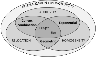
To this end, we will use the axiomatic approach: we will propose several desirable properties and show they imply specific forms of the PEF. Our first two axioms-Normalization and Monotonicity-are satisfied by all functions considered in this paper. The next three axioms-Relocation, Homogeneity and Additivity-taken in pairs, will characterize three classes of PEFs. In Theorem 4, we show that Size and Length are the only functions that satisfy all five axioms.
Our first axiom-Normalization-enforces consistency with the unweighted setting. For unweighted graphs, the path is simply assessed by its size, i.e., its number of edges. Since in the weighted setting unweighted edges are usually treated as edges with weight 1, Normalization states that to a path consisting of k edges of weight 1 should be assigned value k.
Note that Size and Length also coincide for w = (1, . . . , 1).
The second axiom, Monotonicity, states that increasing the length or size of a path should result in a bigger value.
Monotonicity: For every vector w = (w1, . . . , wk)
- f(w) ≤ f((w1, . . . ,wi + ε, . . . ,wk)) for every i ∈ {1, . . . , k} and ε ≥ 0
- f(w) ≥ f((w1, . . . ,wi +wi+1, . . . ,wk)) for every i ∈ {1, . . . , k - 1}
The third axiom, called Relocation, states that the evaluation should depend solely on the size and length of a path. In other words, the distribution of weights in vector w does not affect the evaluation.
Homogeneity, our next axiom, describes how changing the distances affects the evaluation. Specifically, this axiom states that multiplying each value in the vector by a constant, c, affects the evaluation by cα for some α. If α < 1, this notion is consistent with studies that show people tend to map numbers on a logarithmic, and not linear scale [Dehaene et al., 2008].
We will say that a function satisfies α-Homogeneity if it satisfies Homogeneity for a given α.
Our last axiom, Additivity, states that the evaluation of a path combined out of two parts should be equal to the sum of evaluations of both parts considered separately. In other words, the value of a path can be assessed by looking at the value of each its element.
In what follows, we propose three different classes of PEFs that span between Size and Length. Specifically, each of these classes is parametrised by α ∈ [0, 1] that represent the importance of the size of the path, compared to its length. In particular, in each class, for α = 0 we get the Size function and for α = 1 we get the Length function.
Convex Combination path evaluation functions
This class consists of PEFs that for some α ∈ [0, 1] equal:
Thus, each function in this class is simply the convex combination of Size and Length. Theorem 1 shows that if PEF satisfies Normalization, Monotonicity, Relocation, and Additivity, then it must belong to this class.
Theorem 1. The Convex Combination PEFs are the only functions that satisfy Normalization, Monotonicity, Relocation and Additivity.
Proof. The Convex Combination PEFs satisfy Normalization, Monotonicity, Relocation and Additivity. Assume f satisfies Normalization, Monotonicity, Relocation and Additivity. We will prove that it satisfies (1) for some α ∈ [0, 1]. Fix vector w = (w1, . . . , wk). From Relocation and Additivity:
Moreover, from Additivity we know that
Let us consider k = 2. Combining (2) and (3), we get that f((x)) + f((y)) = 2 · f(( x+y 2 )) for every x, y ∈ R+. Based on Cauchy's functional equation we get that f((x)) = α · x + β for every x ∈ R+ and some α, β ∈ R. In result, from Relocation and Additivity we get: f (w) = α·∑ki=1 wi+β ·k. Finally, fromNormalization: f((1, . . . , 1))=k · (α+β)=k, that implies β = 1 - α. Moreover, Monotonicity implies α ∈ [0, 1]. This concludes the proof of Theorem 1.
Exponential path evaluation functions
A function belongs to this class if for some α ∈ [0, 1] equals:
This class was proposed by Opsahl et al. [2010]. In the axiomatization of this class, compared to Convex Combination PEFs, instead of Relocation we use Homogeneity.
Theorem 2. The Exponential PEFs are the only functions that satisfy Normalization, Monotonicity, Homogeneity and Additivity.
Proof. The Exponential PEFs satisfy Normalization, Monotonicity, Homogeneity and Additivity. Assume f satisfies Normalization, Monotonicity, α-Homogeneity for some α ∈
R and Additivity. We will prove that function f satisfies (4). Fix vector w = (w1, . . . ,wk). From Additivity we get that f(w) = f((w1)) + . . . + f((wk)). Now, for each i ∈ {1, . . . , k} from α-Homogeneity we have f((wi)) = wα i · f((1)). Thus, α-Homogeneity and Additivity implies f (w) = (∑ki=1 wα i ) · f((1)). From Normalization, we have f((1)) = 1. Finally, since xα ≤ (x+ ε)α for ε ≥ 0 iff α ≥ 0 and xα + yα ≥ (x + y)α iff α ≤ 1, we get that f satisfies Monotonicity iff α ∈ [0, 1]. This concludes the proof of Theorem 2.
Geometric path evaluation functions
Our third class consists of functions that for some α ∈ [0, 1] have the form
This class does not satisfy Additivity, but satisfies both Relocation and Homogeneity.
Theorem 3. The Geometric PEFs are the only functions that satisfy Normalization, Monotonicity, Relocation and Homogeneity.
Proof. It is easy to check that the Geometric PEFs satisfy Normalization, Monotonicity, Homogeneity and Relocation. Assume f satisfies Normalization, Monotonicity, Relocation and α-Homogeneity for some α ∈ R. We will prove that f satisfies (5). Fix vector w = (w1, . . . ,wk) and assume ∑ki=1 wi = d. Relocation implies that changing consecutive values in the vector w is possible as long as their sum remains the same. In particular, we obtain a vector whose all values are equal. By using α-Homogeneity we get: f(w) = f((d/k, d/k, . . . , d/k)) = (d/k)α ·f(1, . . . , 1). From Normalization, we get (5) for arbitrary α ∈ R. Since dα ≤ (d+ε)α for ε ≥ 0 iff α ≥ 0 and k(1-α) ≥ (k-1)(1-α) iff α ≤ 1, we get that f satisfies Monotonicity iff α ∈ [0, 1]. This concludes the proof of Theorem 3.
Size and Length
Borderline cases for each class are the two standard PEFsSize and Length. This implies they satisfy all five axioms: Normalization, Monotonicity, Relocation, Homogeneity, and Additivity. In the following theorem, we show they are the only such functions.
Theorem 4. Size and Length are the only PEFs that satisfy Normalization, Monotonicity, Relocation, Homogeneity, and Additivity.
Proof. From Theorems 1, 2 and 3 we know that Size and Length satisfy Normalization, Monotonicity, Relocation, Homogeneity, and Additivity.
Assume f is a PEF that satisfies Normalization, Monotonicity, α-Homogeneity, Relocation and Additivity. Let us consider vector w = (x). From Theorem 1, we know f (w) = α · x+(1-α). Analogously, from Theorem 2 and 3, we know that f(w) = xα. Combining these two formulas, we get that α satisfies α · x+(1-α) = xα for every x ∈ R+. For x = 2 we get 1+α = 2α. Since 1+α is a linear function, and 2α is convex or concave, there are at most two solutions. Since α = 0 and α = 1 are solutions, we get they must be the only solutions. In result, only Size and Length satisfy all five axioms. This concludes the proof of Theorem 4.
Figure 1 illustrates the theoretical results of this section.
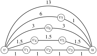
Example 1. Consider the graph from Figure 2. There are 5 paths between v and u: p1, . . . , p5. Paths are ordered ascending by the length and descending by the size.
Clearly, according to Length path p1 with ω(p1) = (1, 1, 1, 1) is the shortest one: f l (ω(p1)) = 4. On the other hand, according to Size path p5 with ω(p5) = (13) is the shortest one: f s (ω(p5)) = 1. Now, consider Convex Combination, Exponential and Geometric PEFs for α = 0.5.
For Convex Combination PEF, we get that f c (w) = ((∑ki=1 wi) + k)/2 is the arithmetic average of Size and Length. Thus, a path with the size larger by one is equivalent to a path with Length larger by one. In result, path p2 with ω(p2)=(1.5, 1.5, 1.5) is the shortest one: f c (ω(p2)) = 3.75.
For Geometric PEF, we get that f g (w) = ((∑ki=1 wi) · k)1/2 is the geometric average of Size and Length. Thus, a path with the doubled Size is equivalent to a path with doubled Length. In result, path p3 with ω(p3) = (3, 3) is the shortest one: f g (ω(p3)) ≈ 3.46.
Finally, consider the Exponential PEF. Here, we get that f e (w) = ∑ki=1 w1/2 i . Compared to Geometric PEF, Exponential PEF favors paths with the greater spread of weights. In result, path p4 with ω(p4) = (6, 1) is the shortest one: f e (ω(p4)) ≈ 3.45.
4 CentralityMeasures forWeighted Graphs
In this section, we show how standard centrality measures can be extended to weighted graphs by using a specific PEF.
We begin with the definition of distance based on such a specific function.
Definition 2. (f-distance) For a PEF, f, f-distance is a function df : G V ×V ×V → R that assigns to every two nodes v, u ∈ V in a graph, G = (V,E, ω), a real value, denoted dfG(v, u), defined as follows:
We assume dfG(v, u) = ∞ if Π(v, u) = ∅, and dfG(v, v) = 0. The f-distance is formally a distance: it satisfies nonnegativity (f returns only positive values), symmetry (graph is undirected) and reflexivity (from the definition). However, it is not always a metric, since it can violate triangle inequality (in fact, if f satisfies Additivity, then f-distance is a metric).
4.1 Degree Centrality
In unweighted graphs, the Degree Centrality simply counts the number of links. In weighted graphs, where weights represent distance between nodes, the number of links contribute positively to node's centrality, but weights of edgesnegatively. To cope with this problem, for an arbitrary PEF, f, graph G = (V,E, ω) and node v ∈ V such that NG(v) = {u1, u2, . . . , uk} we define the Degree Centrality for weighted graphs as follows:
From the technical point of view, in this definition the Degree Centrality is the result of PEF for a path that consists of edges to neighbours of v, but with the weights inversed. Thus, PEF is applied to edges that do not form a path. The rationale behind this is as follows. PEFs aim at finding balance between the number of edges on a path and their weights. The Degree Centrality for weighted graphs has exactly the same goal, but for edges of a node. In result, PEFs and the Degree Centrality have many similarities. For example, in unweighted case, they both simplify to the number of edges. This connection is especially visible for PEFs that satisfy Additivity, where each link is considered separately. The main difference, however, lays in Monotonicity: the bigger weight corresponds to the higher path evaluation, but should result in the lower importance of a node.
For example, for the Geometric PEF we get:
4.2 Closeness and Betweenness Centralities
Since the Closeness and Betweenness Centralities explicitly depend on distances to other nodes, they can be directly translated to weighted graphs as follows:
4.3 Additive Distance-Based Centralities
In unweighted graphs, each additive distance-based centrality is defined by a sequence, a = (a1, a2, . . . , a∞). In weighted graphs, distance can be any real value; thus, instead of a discrete sequence, we use a continuous function, a : R+ → R+. In general, an additive distance-based centrality based on a is defined as follows:
As discussed in [Skibski and Sosnowska, 2018], function a should satisfy a(1) = 1, and a(x) ≥ a(y) for x, y ∈ R+ such that x ≤ y. By using a(x) = 1/x and a(x) = δx for some δ ∈ (0, 1), we get the Harmonic and Decay Centralities:
In a similar fashion, we can define k-Step Reach Centrality:
To give an example, for the graph that represents the map of public transport and f equal to Size or Length, k-Step Reach Centrality can capture number of places that can be reached by a direct connection or in 30 minutes.
5 Experimental Analysis
This section illustrates concepts proposed in this paper.
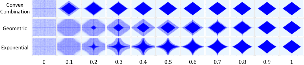
Random Grid: To visualize the difference of three classes of PEFs, we present their performance on random graphs on grids. Specifically, we generated 75 random graphs based on 2-dimensional grids [0, 80] × [0, 80]. Here, every cell is a node in the graph and only cells in the same column or row are connected by an edge. Each edge is created with the probability 0.25 and its weight is the Cartesian distance between those cells. In so doing, we obtained graphs with 6561 nodes, where each cell had on average 70 edges.
For a considered PEF, f, in every graph we selected 30% of nodes closest to the center cell, (40, 40), according to fdistance. Then, we combined all these selected nodes on a single grid. Figure 3 shows the final results for Convex Combination, Geometric, and Exponential PEFs parametrised by α ∈ {0, 0.1, . . . , 0.9, 1.0}. The intensity of color illustrates the percentage of graphs in which a given node was selected.
For each class of PEFs we can see its transition between its border cases-Size (α = 0) and Length (α = 1). The class of Convex Combination PEFs very quickly becomes almost identical to Length. This is because, for most paths in the graph, its Length dominates its Size (in our graphs, all paths had the Size smaller than 13, while the Length was often larger than 50). The transitions of Geometric and Exponential PEFs are much smoother. The Geometric PEFs treat each node at a given distance from the center cell equally-on average, the path to each such a point has the same Size and Length. Thus, from Relocation we should expect the same result. Differently, the Exponential PEFs scales each distance on the path. In result, edges of the darkest area are determined by the functions xα + yα = c for some c ∈ R.
This visualization was inspired by the work by Faliszewski et al. [2017] concerning multiwinner elections rules.
Public transport: As a sample application of centrality measures for weighted graphs, we have considered the graph of public transport of Warsaw, Poland. Here, nodes represent the stops, and edges-a direct connection by bus, tram or metro line during a day. The weight of an edge equals the duration of the fastest connection between its ends. The resulting graph contains 1478 nodes and 116 921 edges.
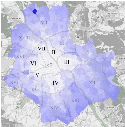
For every centrality measure, Table 1 presents the top districts based on the average value of centralities of stops within. Each centrality measure captures a different property: the Degree Centrality ranks places based on the number of fast direct connections; the Closeness Centrality evaluates places looking on how fast we can get to any other place in the city; finally, the Betweenness Centrality rewards places with more possibilites to transfers. Srodmiescie (I), which is ranked first according to all centralities, is considered to be the center of Warsaw (see Figure 4). Interestingly, Praga Pd. and Praga Pn., that are on the east side of Vistula take very high places in all rankinga. The reason for that may be the high level of routes that go through the bridges that connect west and east sides of city.
Additionally, on Figure 4 we present a Voronoi diagram with stops as the seeds. Specifically, a Voronoi diagram is a partition of the plane into regions based on distance to the specified set of points, called seeds. Each region contains one seed and all points for which this is the closest seed. The color of each region represents the value of the Closeness Centrality for Geometric PEF with parameter α = 0.5. The more blue the region is, the lower its centrality is.
| Degree | Closeness | Betweenness | |
|---|---|---|---|
| 1 | Srodmiescie (I) | Srodmiescie (I) | Srodmiescie (I) |
| 2 | Praga Pd. (III) | Praga Pn. (II) | Praga Pn. (II) |
| 3 | Mokotow (IV) | Ochota (V) | Zoliborz (VII) |
| 4 | Ochota (V) | Praga Pd. (III) | Mokotow (IV) |
| 5 | Zoliborz (VII) | Wola (VI) | Praga Pd. (III) |
6 RelatedWork
There were several attempts in the literature to extend classical centralities to weighted graphs and most of them focus only on the sum of weights [Barrat et al., 2004; Brandes, 2001; Newman, 2001].
Opsahl et al. [2010] proposed the first generalization of the classical centrality measures that takes into account both sum of weights and the number of edges. This class in our paper is introduced under the name Exponential PEF. Candeloro et al. [2016] defined two generalizations of the Degree Centrality. The first one, WDC, is based on the distribution of edge weights. The second one, WSC, is a geometric mean of the sum of weights and the number of edges. Thus, it is equivalent to Degree Centrality for Geometric PEF with parameter α = 0.5 from our paper.
More recently, Stai et al. [2017] considered computational properties of distance-based centrality measures. Cheng et al. [2015] proposed new centrality measures for the analysis of transportation networks. However, they depend not only on the graph, but also additional information, such as the number of passengers. The axiomatic characterization of the class of distance-based centralities for unweighted graphs has been recently proposed by Skibski and Sosnowska [2018]. For the axiomatic characterization of different classes of centralities see, e.g., [Skibski et al., 2018].
7 Conclusions
In this paper, we studied the problem of evaluating arbitrary path in a weighted graph in which weights represent distance between nodes. Using the axiomatic approach, we proposed three classes, parametrised by α ∈ [0, 1], that span between Size and Length. Building upon this analysis, we proposed a way to extend several classical centrality measures to weighted graphs. In our future work, we plan to use our analysis to compare the public transport from different cities. Also, we are interested in creating explicit axiomatic characterization of centrality measures based on discussed PEFs.
Acknowledgments
Jadwiga Sosnowska and Oskar Skibski were supported by the Foundation for Polish Science within the Homing programme (Project title: "CentralityMeasures: fromTheory to Applications").
@inproceedings{ijcai2018p536,
  title     = {Path Evaluation and Centralities in Weighted Graphs - An Axiomatic Approach},
  author    = {Sosnowska, Jadwiga and Skibski, Oskar},
  booktitle = {Proceedings of the Twenty-Seventh International Joint Conference on
               Artificial Intelligence, {IJCAI-18}},
  publisher = {International Joint Conferences on Artificial Intelligence Organization},
  editor    = {Jérôme Lang},
  pages     = {3856--3862},
  year      = {2018},
  month     = {7},
  note      = {Main track},
  doi       = {10.24963/ijcai.2018/536},
  url       = {https://doi.org/10.24963/ijcai.2018/536},
}
TY - CPAPER TI - Path Evaluation and Centralities in Weighted Graphs - An Axiomatic Approach AU - Sosnowska, Jadwiga AU - Skibski, Oskar T2 - Proceedings of the Twenty-Seventh International Joint Conference on Artificial Intelligence, IJCAI-18 PB - International Joint Conferences on Artificial Intelligence Organization PY - 2018 SP - 3856 EP - 3862 DO - 10.24963/ijcai.2018/536 UR - https://doi.org/10.24963/ijcai.2018/536 ER -Copied
Machine-readable versions of this paper, for tools and AI agents:





