
Integrative Network Embedding via Deep Joint Reconstruction
Proceedings of the Twenty-Seventh International Joint Conference on Artificial Intelligence. Main track. Pages 3407-3413.
https://doi.org/10.24963/ijcai.2018/473
Keywords
- Machine Learning Applications: Networks
- Multidisciplinary Topics and Applications: AI and the Web
Abstract
Network embedding is to learn a low-dimensional representation for a network in order to capture intrinsic features of the network. It has been applied to many applications, e.g., network community detection and user recommendation. One of the recent research topics for network embedding has been focusing on exploitation of diverse information, including network topology and semantic information on nodes of networks. However, such diverse information has not been fully utilized nor adequately integrated in the existing methods, so that the resulting network embedding is far from satisfactory. In this paper, we develop a weight-free multi-component network embedding approach by network reconstruction via a deep Autoencoder. Three key components make our new approach effective, i.e., a uniformed graph representation of network topology and semantic information, enhancement to the graph representation using local network structure (i.e., pairwise relationship on nodes) by sampling with latent space regularization, and integration of the diverse information in graph forms in a deep Autoencoder. Extensive experimental results on seven real-world networks demonstrate a superior performance of our method over nine state-of-the-art methods for embedding.
- [Bernardes et al., 2015] Daniel Bernardes, Mamadou Diaby, Raphaël Fournier, Franc ¸oise FogelmanSoulié, and Em- manuel Viennet. A social formalism and survey for rec- ommender systems. SIGKDD, 16(2):20-37, 2015.
- [Cao et al., 2015] Shaosheng Cao, Wei Lu, and Qiongkai Xu. Grarep: Learning graph representations with global structural information. In CIKM, pages 891-900, 2015.
- [Cui et al., 2017] Peng Cui, Xiao Wang, Jian Pei, and Wenwu Zhu. A survey on network embedding. arXiv:1711.08752, 2017.
- [Groth et al., 2013] Detlef Groth, Stefanie Hartmann, Sebas- tian Klie, and Joachim Selbig. Principal components anal- ysis. Computational Toxicology, 930:527-547, 2013.
- [Grover and Leskovec, 2016] Aditya Grover and Jure Leskovec. Node2vec: Scalable feature learning for networks. In SIGKDD, pages 855-864, 2016.
- [He et al., 2017] Dongxiao He, Zhiyong Feng, Di Jin, Xi- aobao Wang, and Weixiong Zhang. Joint identification of network communities and semantics via integrative mod- eling of network topologies and node contents. In AAAI, pages 116-124, 2017.
- [Huang et al., 2017] Xiao Huang, Jundong Li, and Xia Hu. Accelerated attributed network embedding. In ICDM, pages 633-641, 2017.
- [Kim, 2014] Yoon Kim. Convolutional neural networks for sentence classification. arXiv:1408.5882, 2014.
- [Liao et al., 2017] Lizi Liao, Xiangnan He, Hanwang Zhang, and Tat-Seng Chua. Attributed social network embedding. arXiv:1705.04969, 2017.
- [Liu et al., 2012] Haifeng Liu, Zhaohui Wu, Xuelong Li, Deng Cai, and Thomas S Huang. Constrained nonnega- tive matrix factorization for image representation. IEEE Trans. Patt. Anal. Mach. Intell., 34(7):1299-1311, 2012.
- [Liu et al., 2017] Yang Liu, Zhonglei Gu, Yiu-ming Cheung, and Kien Hua. Multi-view manifold learning for media in- terestingness prediction. In ICMR, pages 308-314, 2017.
- [Newman, 2006] Mark Newman. Modularity and commu- nity structure in networks. PNAS, 103(23):8577-8582, 2006.
- [Pan et al., 2016] Shirui Pan, Jia Wu, Xingquan Zhu, Chengqi Zhang, and Yang Wang. Tri-party deep network representation. Network, 11(9):12, 2016. IJCAI
- [Perozzi et al., 2014] Bryan Perozzi, Rami Alrfou, and Steven Skiena. Deepwalk: online learning of social rep- resentations. In KDD, pages 701-710, 2014.
- [Ruan et al., 2010] Jianhua Ruan, Angela K Dean, and Weixiong Zhang. A general co-expression network-based approach to gene expression analysis: comparison and ap- plications. Bmc Systems Biology, 4(1):8, 2010.
- [Ruan et al., 2013] Yiye Ruan, David Fuhry, and Srinivasan Parthasarathy. Efficient community detection in large net- works using content and links. In WWW, pages 1089- 1098, 2013.
- [Shi and Malik, 2000] Jianbo Shi and Jitendra Malik. Nor- malized cuts and image segmentation. IEEE Trans. Patt. Anal. Mach. Intell., 22(8):888-905, 2000.
- [Tang et al., 2015] Jian Tang, Meng Qu, Mingzhe Wang, Ming Zhang, Jun Yan, and Qiaozhu Mei. Line: Large- scale information network embedding. In WWW, pages 1067-1077, 2015.
- [Tu et al., 2017] Cunchao Tu, Han Liu, Zhiyuan Liu, and Maosong Sun. Cane: Context-aware network embedding for relation modeling. In ACL, pages 1722-1731, 2017.
- [Tu et al., 2018] Ke Tu, Peng Cui, Xiao Wang, Fei Wang, and Wenwu Zhu. Structural deep embedding for hyper- networks. In AAAI, 2018.
- [Wang et al., 2016] Daixin Wang, Peng Cui, and Wenwu Zhu. Structural deep network embedding. In SIGKDD, pages 1225-1234, 2016.
- [Wang et al., 2017] Xiao Wang, Peng Cui, Jing Wang, Jian Pei, Wenwu Zhu, and Shiqiang Yang. Community preserv- ing network embedding. In AAAI, pages 203-209, 2017.
- [Yang et al., 2015] Cheng Yang, Zhiyuan Liu, Deli Zhao, Maosong Sun, and Edward Y Chang. Network represen- tation learning with rich text information. In IJCAI, pages 2111-2117, 2015. IJCAI
- [Yin et al., 2012] Chunxia Yin, Qinxe Peng, and Tao Chu. Personal artist recommendation via a listening and trust preference network. Phys. Stat. Mech. Appl., 391(5):1991- 1999, 2012.
References were extracted automatically from the PDF and may contain errors.
Full text extracted automatically from the PDF; figures, tables and equations may differ. The PDF is the version of record.
1 Introduction
Network embedding (NE) aims to encode a network in a low dimensional vector representation for each node in the network so as to extract intrinsic features of the network. NE has been adopted to solve many real-world problems, such as link prediction, user recommendation and community detection [Wang et al., 2016; Tu et al., 2018]. Network topology is the most common representation of a network. Recently, many NE methods using network topology alone have been proposed, as reviewed in [Cui et al., 2017].
† Both authors contributed equally to this work.
∗ Corresponding author.
However, in many networks in the real life, there are often two types of information which can be exploited in NE, i.e., network topologies and semantic or content information on nodes of a network. While network topology, typically in the form of node adjacency matrix, is the most common form of network representation, semantic information has also gained popularity in various application domains [He et al., 2017]. For example, text messages and multimedia information, including images and sound bites, are ubiquitous in social networks, e.g., Facebook and Twitter, describing the contents of nodes. Semantic information often carries orthogonal and complementary knowledge beyond node connectivity and topology of a network. Incorporating semantic information is expected to significantly enhance NE based on network topology alone.
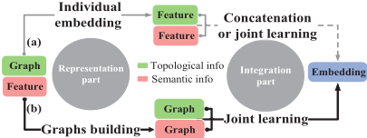
The existing methods for NE follow a common approach when using both topological and semantic information (Fig. 1(a)). In this approach, network topology is first converted into a feature representation, which is then used to embed the network topological structures into a low dimensional space.
Semantic information on nodes, in a feature representation, is also used to derive low-dimensional embedding on node semantics. All these NEs are then concatenated to joint learn the final embedding (Fig. 1(a)). For example, the TADW method [Yang et al., 2015] employs a matrix factorization based DeepWalk [Perozzi et al., 2014] with text information to generate individual embedding of topology and semantic content, and concatenate them to form the final embedding. The SNE method [Liao et al., 2017] projects the one-hot topological representation to a dense vector representation, encodes the semantic features to generate a compact vector, and then concatenates them to jointly learn a node embedding. The CANE method [Tu et al., 2017] captures the structure-based embedding from topology and obtains textbased embedding via convolutional neural networks [Kim, 2014], and concatenates these two to form a final embedding.
Although they have achieved reasonable results, the existing methods have three drawbacks, in which the first two refer to representation of different types of components and third refers to integration. First, a key step of these NE methods is to represent network topological information using a feature vector representation. Different from semantic information on nodes, network topology information explicitly specifies relational structures among the nodes in a network. When converted into a feature vector representation, such relational information may be lost or may not be faithfully represented, resulting in poor NE. The second drawback of the existing methods is in the way that they treat the semantic information. Specifically, content information is typically better to be considered to lie in some kind of non-linear manifolds [Liu et al., 2017]. However, the existing methods only focus on the global linear relations among data points in the input space and fail to honor the non-linear relationship among network data points. The third drawback of the existing methods is that they do not truly integrate the two different types of information (i.e., the information of network topology and semantic information on nodes) that should be fully utilized for NE. They combine each individual topological feature vector and semantic feature vector together to learn the corresponding embedding. In essence, the individual feature vector only contains individual information without inter-individual association relationships, so that the integration is unsatisfactory to explore and exploit the complementary relationship between these two types of information, making their results inaccurate on many real applications.
To overcome the problems of the existing methods, we propose a novel Unified Weight-free Multi-component Network Embedding (UWMNE) approach via a joint network reconstruction using deep Autoencoder (Fig. 1(b)). In our approach, we first use graphs as a uniform representation scheme to represent both network topologies and semantics. This was inspired by the intuition that graph is a more potent representation vehicle than vector representation in preserving structural and relational features of a network. Graph is also able to better describe the geometry of the latent local manifolds underlying semantic information. This is analogous to the ideas of spectral methods (e.g., normalizedcut [Shi and Malik, 2000] and modularity spectra [Newman, 2006]), which also use a graph representation before learning features. Similarly, in the representation part we maintain network topologies in the graph form and build neighborhood graphs to represent semantics. Benefited from the uniform graph representation for the multiple types of network topological and semantic information, we then in the integration part use deep neural networks to integrate the topological and semantic information in these graphs to learn a unified network embedding. Our method is thus able to accommodate non-linear manifolds of semantic information, support crosslearning by integrating both topological and semantic information in one platform of neural networks, and maintain a balance between different components of the network representation. To further improve the performance of embedding, we extend the basic UWMNE method to include a local enhancement (UWMNE-LE), which combines link strength and semantic similarity between nodes to build pairwise constraints and introduce a graph regularization based on pairwise constriants to reinforce the local structure consistency.
2 The Approach
We first give an overview to our new approach, and then present the basic model UWMNE along with its optimization, and finally introduce a local enhancement (UWMNE-LE).
2.1 Overview
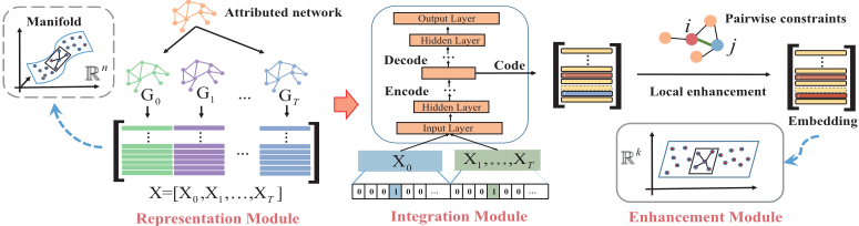
The overall structure and three major modules of our new NE learning method is illustrated in Fig. 2. The three modules, from left to right of the figure, are introduced to extract network features from topology and semantic information, to combine topology and semantics using a deep Autoencoder, and to enhance the learning by exploiting local network structures (i.e., pairwise relationship on nodes).
In the representation module, we maintain the network topology in the graph form and represent semantic content by rank-based similarity graphs. In building a similarity graph, cosine similarity and the k-nearest neighbor method [Ruan et al., 2010] are applied to accommodate some latent non-linear manifold structures underlying the sematic content. Since we expect each data point and its neighbours to lie on a locally smooth manifold, it is convenient to jointly embed all nodes, along with their topologies and semantic information, into a lower dimensional space to unfold the hidden manifold.
In the integration module, an Autoencoder is employed as a compact yet powerful vehicle to integrate information of network topology and semantics. The graphs for network topology and semantic similarity graphs are concatenated into mini-batches and fed into the Autoencoder, which attempts to reconstruct the original graphs of network topology and semantics. The value of the loss function or the overall reconstruction error is then propagated back from the output layer to the input layer to compute the gradients to adjust the parameters of the Autoencoder. When the deep Autoencoder converges, its most inner hidden layer is expected to hold the final joint network embedding.
In addition, to make the network embedding more effective, we further add an enhancement module to reinforce the local structure consistency by incorporating pairwise constraints between nodes. These constraints are constructed by a measure of similarity between two nodes in the network by combining their link strength and semantic similarity. Specifically, link strength is estimated based on whether the link is likely to reside within a group. Semantic similarity is estimated through the cosine similarity. Finally, the pairwise constraints are used to design a graph regularization term, which are then integrated with the loss function to encode the final locally enhanced embedding.
2.2 TheWMCNEModel
Given an undirected and attributed network G = (V,E, T) with n nodes V = {v1, v2, . . . , vn}, m edges E, and T types of attributes t (i.e., semantic data) on nodes, the objective of network embedding is to represent each node vi as a vector hi ∈ Rk of k (k ≪ n) dimension. In the following, we first consider the graph representation of network topology (X0) and the graph representation of each type of node attributes (semantics) (Xt, t = 1, 2, · · · , T).
Network topology G0 = (V,E) can be represented as an n×n matrix X0, including information in the adjacency matrix A = [aij] ∈ Rn×n where aij = 1 if there is an edge between nodes vi and vj. Furthermore, in comparison with the adjacency matrix A, the modularity matrix B [Newman, 2006] includes not only microscopic structural properties on nodes and links in A, but also a higher-order structural property of community structures what are not directly in A. It has been proven that preserving community properties is crucial in network embedding [Wang et al., 2017]. Therefore, we use the modularity matrix B instead of adjacency matrix A as the final representation of network topology, defined as:
where ξi = ∑j aij is the degree of node vi.
For each type of attributes (i.e., semantics) on nodes, we construct a rank-based similarity graph that can be also represented by an n × n matrix Xt ∈ Rn×n , for t = 1, 2, . . . , T . Take a piece of text as an example. Text content on each node (e.g., node vi) can be represented as a vector of bagof-words (e.g., ωi). We calculate the similarity between two nodes in the network to form the similarity graph S = [sij ] = [(ωi · ωj)/(‖ωi‖‖ωj‖)]. We further utilize a k-nearest neighbor method on this similarity graph to select the top-k most similar nodes for each node to form a new sparse graph S as the graph representation for text contents. Moreover, similar to the adjacency matrix A, S does not capture any mesoscopic cluster-structure property. But luckily, the Markov matrix M which is often used in spectral graph theory [Shi and Malik, 2000] contains the cluster-structure property directly. So we use M instead of S as the finally graph representation. Specifically we define
where D = diag(d1, d2, ..., dn) and di = ∑j sij. Also of note, we can use similar ways to define graph representation for other types of semantic attributes though here we only give text content as an example.
By horizontally concatenating all of the matrices of the topology graph and semantic rank-based similarity graphs into a uniformed representation X = [X0,X1, . . . ,XT ], we form the input data to an Autoencoder. Each row of the matrix X (i.e., xi) corresponds to all of the input representations for each node (i.e., vi) in the network. The Autoencoder consists of two structurally symmetric components, the encoder and the decoder. The encoder maps data in the input space to a latent space, and the decoder maps the objects in the latent space to the reconstruction space. Formally, the encoder maps the input data xi into hi in the latent space as:
where W(H) and b(H) are the parameters of the encoder, and f(·) is an encoder activation function, such as sigmoid(x) = 1/(1 + exp(-x)). Likewise, the decoder maps an object hi in the representation space into yi in the reconstruction space as yi = f(W(Y)hi + b(Y) ), where W(Y) and b(Y) are the parameters of the decoder to be learned, and f(·) is a decoder mapping function, which can be the same as the encoder function. The Autoencoder is then trained by minimizing the reconstruction error between the input objects and the reconstructed objects under parameters θ = {W(H) , b(H) , W(Y) , b(Y)}:
The goal of our WMCNE method is then minimize L(X,Y) in Eq. (4), which is achieved by using back propagation algorithm (BP) with stochastic gradient descent, i.e., W ∗ ji = W ∗ ji -α ∂ ∂W ∗ ji L(X, Y), in which ∗ = {(H), (Y)} is a wildcard. By defining z∗ = W∗x + b∗ , we get the gradient of the parameters θ as:
where δ∗ j = ∂L(X,Y)/∂z∗j is an error term that measures the reconstruction error between the activation and the true target value. The update to the error terms are defined as:
where f ′ (·) is the partial derivative of f(·). Once the Autoencoder converges, the representation in the hidden layer is taken as the final embedding of the network.
To better represent these real networks, we stack a series of Autoencoders to construct an overall deep Autoencoder to learn network embedding. Specifically, we train the first Autoencoder to reconstruct input matrix X, and obtain the first latent representation H(1) along with the first reconstructed data Y(1) . We then construct the model layer by layer by training the ith Autoencoder to reconstruct the hidden layer representation of the (i-1)th Autoencoder, and then obtain a new latent representation H(i) . The objective function of the ith layer is finally ˆ θ(i) = arg minθ(i) L(H(i-1) , Y(i) ).
2.3 Local Enhancement - TheWMCNE-LEModel
To enhance local network structures, we first introduce a similarity measure between two nodes to measure the node closeness in the given network. We then incorporate a soft pairwise constraint on nodes and introduce a graph regularization to a local enhancement (WMCNE-LE). The rationale of this enhancement follows the intuition that two nodes should be similar in their low-dimensional embedding space if they are close to each other in the original attributed network.
To measure the node closeness in a network, we introduce a similarity between two nodes by combining their link strength and semantic similarity. Specifically, we adopt the cosine similarity on content to compute the similarity matrix S = [sij] = [cos(ωi, ωj)] where ωi is the content vector for node vi and cos(ωi, ωj) = (ωi ·ωj)/(‖ωi‖‖ωj‖). We then select the top-k similar neighbors for each node to form the set of content edges E c . These content edges E c and the original topological edges E t are combined as a unified set E u . For each node vi and its neighbor vj in E u , we compute their link strength Simt = [Simij t ] = [cos(ai, aj)] and the semantic similarity Simc = [Simij c ] = [sij], where ai is the ith row vector of the adjacency matrix A of the given network.
In order to ensure that the network topology and semantic content are equally important, we combine them into
where z-norm(·) [Ruan et al., 2013] is defined as:
Here we utilize z-norm(·) rather than other normalization, because it has the advantage of being both shift and scale invariant.
Finally, we choose the top-⌈√count(E u i )⌉ neighbors with the highest similarities of each node vi to form a local sampling graph Gsample, where count(E u i ) denotes the number of neighbors of vi in E u . Graph Gsample can be used to describe whether nodes are close or not in the given network.
Given the local sampling graph Gsample, we define a soft pairwise constriant matrix P = [pij] ∈ Rn×n , where pij = 1 if nodes vi and vj have an edge in Gsample, or pij = 0 otherwise. Therefore, given the pairwise constraint matrix and similarity measurement (i.e., Euclidean distance), we can define the pairwise constraint as:
Lreg = Dreg - P, where Dreg = [(dreg)ij] ∈ Rn×n is a diagonal matrix with elements (dreg)ii = ∑nj=1 pij and (dreg)ij = 0 for i ̸= j. We can then incorporate the pairwise constraints as a graph regularization term into the loss function in Eq. (4) to enhance the local network structure of the model, and obtain the overall loss function as:
where β is a trade-off parameter. After training the Autoencoder, W(H) and b(H) are obtained, and then Eq. (3) can be used to generate the new representations for all nodes.
The objective of WMCNE-LE in Eq. (9) can also be optimized by the BP algorithm as before. Since the graph regularization term is independent of the reconstruction matrix, the updating of δ(Y) join will remain the same as updating of δ(Y) in Eq. (6). But the updating of δ(H) join needs to be modified as:
where ⊙ is the element-wise mutliplication.
3 Experimental Validation
To evaluate the effectiveness of our approach WMCNELE, we tested it experimentally on three network applications, i.e., classification, clustering and user recommendation. Seven publicly available datasets with varying sizes and characteristics are used. WebKB, containing 4 sub-datasets, is a web page dataset gathered in four different universities, i.e., Cornell, Texas, Washington and Wisconsin. Citeseer is a citation network, which consists of 3,312 scientific publications from 6 sub-fields with 4,732 citation relationships. UAI2010 contains article information fromEnglishWikipedia pages. It contains 3,067 articles and 45,006 links between documents. Pubmed consists of 19,717 publications in 3 classes.
| Packages / AC (%) | Methods | Cornell | Texas | Washington | Wisconsin | Citeseer | UAI2010 | Pubmed |
|---|---|---|---|---|---|---|---|---|
| LibSVM | DeepWalk | 38.97 | 49.18 | 55.30 | 49.24 | 52.52 | 58.69 | 78.79 |
| Node2Vec | 35.90 | 50.27 | 47.47 | 46.56 | 61.63 | 61.95 | 80.30 | |
| LINE | 43.59 | 68.85 | 59.91 | 54.58 | 41.07 | 52.85 | 75.47 | |
| GraRep | 53.33 | 72.68 | 52.07 | 59.16 | 54.28 | 64.20 | 81.64 | |
| MNMF | 36.92 | 65.03 | 61.29 | 54.20 | 40.29 | 52.17 | 65.19 | |
| TADW | 64.10 | 67.76 | 59.45 | 64.50 | 69.83 | 68.70 | 85.37 | |
| AANE | 51.80 | 56.28 | 64.06 | 43.13 | 24.70 | 41.47 | 78.63 | |
| TriDNR | 37.95 | 48.09 | 47.01 | 40.46 | 54.47 | 57.74 | 79.07 | |
| SNE | 48.21 | 57.92 | 54.38 | 59.54 | 44.74 | 41.18 | 78.37 | |
| WMCNE-LE | 70.76 | 73.22 | 72.81 | 78.63 | 68.86 | 71.47 | 82.07 | |
| DeepWalk | 38.46 | 48.09 | 53.92 | 49.62 | 48.42 | 60.61 | 78.36 | |
| Node2Vec | 37.95 | 50.27 | 45.62 | 46.95 | 52.44 | 60.38 | 81.08 | |
| LINE | 44.10 | 63.39 | 56.22 | 54.96 | 40.56 | 53.93 | 74.92 | |
| GraRep | 53.33 | 69.40 | 51.15 | 60.31 | 53.61 | 63.74 | 81.37 | |
| LibLINEAR | MNMF | 34.87 | 57.38 | 58.53 | 51.15 | 46.42 | 54.06 | 70.41 |
| TADW | 61.03 | 67.76 | 64.98 | 67.56 | 72.53 | 68.50 | 86.80 | |
| AANE | 41.54 | 53.01 | 61.75 | 38.93 | 22.24 | 43.04 | 77.99 | |
| TriDNR | 34.87 | 42.08 | 43.32 | 41.60 | 52.91 | 57.94 | 78.40 | |
| SNE | 45.64 | 59.02 | 55.76 | 59.92 | 44.35 | 29.87 | 77.20 | |
| WMCNE-LE | 68.71 | 73.77 | 75.58 | 80.53 | 68.97 | 69.78 | 82.98 |
We compared WMCNE-LE with nine state-of-the-art methods: 1) Topology-based embedding methods: DeepWalk [Perozzi et al., 2014], Node2Vec [Grover and Leskovec, 2016], MNMF [Wang et al., 2017], LINE [Tang et al., 2015] and GraRep [Cao et al., 2015], and 2) embedding methods using both topological and semantic information: TADW [Yang et al., 2015], SNE [Liao et al., 2017], TriDNR [Pan et al., 2016] and AANE [Huang et al., 2017].
The final embedding dimension are often set to power of 2, while any dimension can be set up in essence. To ensure fair, here we uniformly set it to 64 for all of the methods. The parameters of the methods compared were set to their default values. For our method, we set k = 9 to construct k-nearest neighbor graphs since we often reached stable results when k is from 6 to 9. We also used the Theano deep learning tools to construct stacked Autoencoders with a learning rate of 0.1, and our activation function is sigmoid(·) in the experiment.
3.1 Node Classification
After getting the network embedding, we adopt the LibSVM and LibLINEAR software packages in Weka to classify these nodes with ground-truth. For each network, we used 10-fold cross-validation, and accuracy (AC) [Liu et al., 2012] as the gold metric to evaluate the performance of all methods. The results are shown in Table 3. As shown, our WMCNE-LE method outperformed the methods compared on most networks, except on Citeseer and Pubmed on which WMCNELE ranked the second. In particular, WMCNE-LE outperformed the best baseline method (i.e., GraRep) by 11.5% using LibSVM and 12.5% using LibLINEAR on average.
3.2 Node Clustering
After having the embedding, we applied k-means to the resulting embedding of nodes to cluster them into classes. Here, besides AC we also used NMI (normalized mutual information) [Liu et al., 2012] as an additional accuracy metric since NMI has been used more often in node clustering. Our results (Table 2) show that WMCNE-LE performed the best on 6 of the 7 networks in AC and 5 of the 7 networks in NMI. On average, WMCNE-L improved upon the best baseline (i.e., LINE) by 12.9% (AC) and 19.2% (NMI).
| Metrics (%) | Methods | Cornell | Texas | Washington | Wisconsin | Citeseer | UAI2010 | Pubmed |
|---|---|---|---|---|---|---|---|---|
| DeepWalk | 36.05 | 46.72 | 40.76 | 38.76 | 36.21 | 37.58 | 64.84 | |
| Node2Vec | 33.85 | 47.54 | 37.33 | 49.62 | 40.76 | 36.74 | 66.76 | |
| LINE | 39.49 | 57.38 | 56.68 | 45.43 | 25.01 | 32.07 | 43.11 | |
| GraRep | 31.79 | 36.72 | 31.36 | 33.24 | 31.20 | 37.87 | 54.43 | |
| AC | MNMF | 37.03 | 46.72 | 53.11 | 41.66 | 25.92 | 24.50 | 40.35 |
| TADW | 47.69 | 59.23 | 50.30 | 55.00 | 55.39 | 36.19 | 57.46 | |
| AANE | 37.28 | 30.49 | 41.57 | 30.53 | 21.76 | 17.82 | 34.55 | |
| TriDNR | 38.21 | 47.54 | 43.59 | 43.70 | 34.44 | 35.59 | 59.29 | |
| SNE | 43.08 | 41.53 | 48.80 | 55.50 | 31.17 | 30.70 | 66.13 | |
| WMCNE-LE | 53.35 | 55.64 | 66.39 | 55.98 | 58.46 | 40.17 | 65.60 | |
| DeepWalk | 7.06 | 6.16 | 5.66 | 7.65 | 10.58 | 34.28 | 26.55 | |
| Node2Vec | 6.65 | 4.49 | 2.94 | 7.86 | 12.99 | 33.87 | 25.02 | |
| LINE | 9.27 | 23.16 | 24.95 | 9.39 | 5.62 | 29.01 | 7.17 | |
| GraRep | 8.80 | 12.43 | 5.18 | 8.02 | 9.61 | 33.64 | 17.76 | |
| NMI | MNMF | 11.63 | 17.20 | 22.15 | 10.10 | 8.95 | 19.23 | 1.41 |
| TADW | 11.13 | 10.90 | 11.63 | 17.52 | 31.60 | 37.92 | 20.11 | |
| AANE | 9.55 | 3.52 | 13.19 | 2.86 | 1.19 | 15.49 | 0.01 | |
| TriDNR | 7.20 | 4.32 | 8.10 | 6.60 | 9.59 | 32.37 | 19.28 | |
| SNE | 11.11 | 12.63 | 17.43 | 23.94 | 7.31 | 26.59 | 26.61 | |
| WMCNE-LE | 38.22 | 27.03 | 40.64 | 38.26 | 32.59 | 41.60 | 25.81 |
3.3 User Recommendation
We considered on the shared LASTFM data in HetRec 2011, which consists of 1,892 users and 17,632 artists from an online music system Last.fm. The user-artist relations, represented by the listening counts of a user on all artists. The training data had ∼90% of the user-artist relations after December 2010, and the rest ∼10% were used as the test data.
To evaluate the methods on recommendation, the recommended artist list Ru was derived by a basic collaborative filtering algorithm [Bernardes et al., 2015] as score(u, a) = ∑v∈N(u) w(u, v)rv,a, where w(u, v) is the similarity between users u and v, N(u) is the neighbors of user u, and rv,a = 1 if user v has listened to artist a or 0 otherwise.
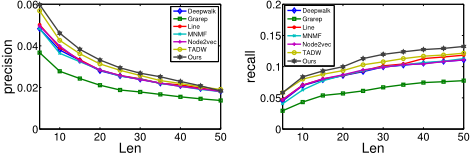
We used precision and recall [Yin et al., 2012] to evaluate the performance of recommendations. The precision and recall of a method compared was averaged over all of the test cases. We varied the number of recommendations from 5 to 50. The results are shown in Fig. 3. As shown, our WMCNELE prevailed over all baseline methods in both precision and recall. This further demonstrated that WMCNE-LE is also effective in integrating multiple component embeddings to obtain high-quality representations using attributed networks for the prediction task.
4 Why Our ApproachWorks
Our new approach WMCNE-LE has four eminent features, a uniform graph representation for topological and semantic information, a parameter-free data integration via Autoencoder, a deep Autoencoder structure, and preservation of network local structures. Here we analyze the effects of these features.
http://ir.ii.uam.es/hetrec2011
| Metrics (%) | Representation Combinations | Citeseer | UAI2010 | Pubmed |
|---|---|---|---|---|
| AC | A + C PCA(A) + C A + S | 39.88 40.94 40.98 | 28.85 | 48.75 48.14 45.71 |
| 28.72 | ||||
| 37.08 | ||||
| B + M | 58.46 | 40.17 | 59.60 | |
| NMI | A + C | 18.88 | 24.35 | 14.78 |
| PCA(A) + C | 18.69 | 23.78 | 14.42 | |
| A + S | 19.22 | 39.24 | 17.51 | |
| B + M | 32.59 | 41.60 | 24.81 |
4.1 Graph Representations
Recall our main idea illustrated in Fig. 1(b). To evaluate the effectiveness of using graphs rather than feature vectors for data representation, we modeled and compared the combination of network topology and semantic information (e.g., text content) in four ways. 1) A + C: The adjacancy matrix A and text content feature matrix C are concatenated directly as input representation. 2) PCA(A) +C: Network topology is embeded in a lower dimensional space via PCA (Principal Component Analysis) [Groth et al., 2013], and then concatenated with text content as the input representation. 3) Our A+S: The similarity matrix S is calculated by the cosine similarity and the k-nearest neighbor method, and then concatenated with the adjacency matrix A as the input representation. 4) Our final B+M: The modularity matrix B and Markov matrixMare calculated by Eq. (1) and Eq. (2), respectively, and then concatenated to form the input representation.
A comparison of these ways of combinations showed that the combinations of "A+C" and "B+M" have a much better performance than the remaining two (Table 3). To be specific, "A + C" is a direct combination of different types of input data. "PCA(A) + C" performs a joint learning over individual embedding, which is often adopted in the existing methods. However, it destroys the association relationships among nodes of the original network, which weakens its performance. Our "A+C" delivered some better results, because the graph representation preserves the relationship of network nodes and better describes the (latent) local manifold geometry hidden in semantic content. Our improved "B+M" method achieves the best performance. The modularity matrix B contains some higher-order community properties beyond for network topology and Markov matrix M captures content clusters, which in combination make our approach effective by truly integrating topological and semantic information in one computational platform of Autoencoder.
4.2 Parameter-free Data Integration
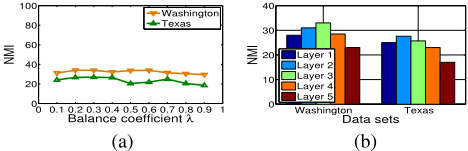
To analyze the automatic-weighting property of our basic WMCNE method, we carried out a balance experiment on two sample datasets (i.e., Texas and Washington). We concatenated the modularity matrix B and the Markov matrix M with a balance coefficient λ to adjust the input data X = [λB, (1-λ)M] to the Autoencoder. We varied λ from 0.1 to 0.9 with an increment 0.1, and trained the model with different λ. We then reported the average result over 10 random initializations (Fig. 4(a)). As shown, varying λ has little influence. In particular, the overall variances are 0.026% on Washington and 0.087% on Texas, which are all less than 0.1%. In
80
60
40
20
0
Without enhance
With enhance
Cor Tex Was Wis Cit UAI Pub
Data sets
(a)
summary, this experiment reveals that the Autoencoder based data integration can determine balances of different data.
4.3 Deep Architecture
To appreciate the advantage of the deep architecture of the Autoencoder in WMCNE, we trained the Autoencoder with different number of layers on Washington and Texas datasets (Fig. 4(b)). The performance of WMCNE improves as the number of layers increases initially and then, as expected, degenerates when too many layers are added (Fig. 4(b)).
Two possible reasons are behind the performance improvements gained when the number of layers initially increases. First, the document networks and social networks have multilevel modalities, i.e., document, topic, words, etc. Real-world networks often have various non-linear features, i.e., a relationship among users is not necessarily linear. In comparison to existing methods with one layer of representation, our method can learn deep multi-levels representations. Second, our method integrates multiple data types without additional weights and automatically learns parameters to improve performance. When too many layers are stacked, the input data are mapped further to a lower dimensional space, which may cause a loss of useful information in the original data.
4.4 Preservation of Local Network Structure
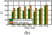
We examined the effectiveness of our local structure enhancement. We compared the vanilla WMCNE and its enhanced version WMCNE-LE on all data sets for both node classification and node clustering (Fig. 5). WMCNE-LE consistently outperformed WMCNE. Specifically, for node clusteing, WMCNE-LE improved upon WMCNE by 10.2% in AC on average. For node classification, the improvements are 10.5% using software packages LibLINEAR in terms of AC on average. The result showed that incorporating local network structure into node embedding helps to learn better node embedding for network analysis.
AC
5 Conclusion
We proposed a novel network embdding approach to integrate topological and semantic network information. Comparing to the existing methods, our new approach has four distinctive features. First, it adopts a uniform graph representation for topological and semantic information. Using graph can overcome the drawback of breaking association relationships among network objects that are typically represented in network topologies. Second, it is a parameter-free approach to adequately integrate data from diverse sources and of different types. This feature is supported by the uniform graph representation and the Autoencoder used for data integration. By putting all types of data into one integration platform, learning across different data sources (aka, cross learning) can be readily achieved. Third, it exploits deep neural network architecture in Autoencoder so that deep, multi-level, non-linear latent features in network data can be explored. Fourth, it preserves network local structures so that complex manifold in network data, particularly semantic information, can be fully utilized in network embedding. Extensive experimental results showed a superior performance of our new approach.
Acknowledgments
The work was supported by Natural Science Foundation of China (61502334, 61772361, 61503281), National Key R&D Program of China (2017YFC0820106) and Elite Scholar Program of Tianjin University (2017XRG-0016).
@inproceedings{ijcai2018p473,
  title     = {Integrative Network Embedding via Deep Joint Reconstruction},
  author    = {Jin, Di and Ge, Meng and Yang, Liang and He, Dongxiao and Wang, Longbiao and Zhang, Weixiong},
  booktitle = {Proceedings of the Twenty-Seventh International Joint Conference on
               Artificial Intelligence, {IJCAI-18}},
  publisher = {International Joint Conferences on Artificial Intelligence Organization},
  editor    = {Jérôme Lang},
  pages     = {3407--3413},
  year      = {2018},
  month     = {7},
  note      = {Main track},
  doi       = {10.24963/ijcai.2018/473},
  url       = {https://doi.org/10.24963/ijcai.2018/473},
}
TY - CPAPER TI - Integrative Network Embedding via Deep Joint Reconstruction AU - Jin, Di AU - Ge, Meng AU - Yang, Liang AU - He, Dongxiao AU - Wang, Longbiao AU - Zhang, Weixiong T2 - Proceedings of the Twenty-Seventh International Joint Conference on Artificial Intelligence, IJCAI-18 PB - International Joint Conferences on Artificial Intelligence Organization PY - 2018 SP - 3407 EP - 3413 DO - 10.24963/ijcai.2018/473 UR - https://doi.org/10.24963/ijcai.2018/473 ER -Copied
Machine-readable versions of this paper, for tools and AI agents:





