
Predicting Complex Activities from Ongoing Multivariate Time Series
Proceedings of the Twenty-Seventh International Joint Conference on Artificial Intelligence. Main track. Pages 3322-3328.
https://doi.org/10.24963/ijcai.2018/461
Keywords
- Machine Learning Applications: Other Applications
- Multidisciplinary Topics and Applications: Ubiquitous Computing Systems
Abstract
The rapid development of sensor networks enables recognition of complex activities (CAs) using multivariate time series. However, CAs are usually performed over long periods of time, which causes slow recognition by models based on fully observed data. Therefore, predicting CAs at early stages becomes an important problem. In this paper, we propose Simultaneous Complex Activities Recognition and Action Sequence Discovering (SimRAD), an algorithm which predicts a CA over time by mining a sequence of multivariate actions from sensor data using a Deep Neural Network. SimRAD simultaneously learns two probabilistic models for inferring CAs and action sequences, where the estimations of the two models are conditionally dependent on each other. SimRAD continuously predicts the CA and the action sequence, thus the predictions are mutually updated until the end of the CA. We conduct evaluations on a real-world CA dataset consisting of a rich amount of sensor data, and the results show that SimRAD outperforms state-of-the-art methods by average 7.2% in prediction accuracy with high confidence.
- [Anderson et al., 2012] H. S Anderson, N. Parrish, K. Tsukida, and M. R Gupta. Reliable early classi- fication of time series. In Proceedings of ICASSP, pages 2073-2076, 2012.
- [Chollet and others, 2015] Franc ¸ois Chollet et al. Keras. https://github.com/keras-team/keras, 2015. Link
- [Dachraoui et al., 2015] A. Dachraoui, A. Bondu, and A. Cornuéjols. Early classification of time series as a non myopic sequential decision making problem. In Proceed- ings of ECML-PKDD, pages 433-447, 2015.
- [Fan et al., 2016] X. Fan, H. Zhang, C. Leung, and C. Miao. Comparative study of machine learning algorithms for ac- tivity recognition with data sequence in home-like envi- ronment. In Proceedings of MFI, pages 168-173, 2016.
- [Ghalwash and Obradovic, 2012] M. F Ghalwash and Z. Obradovic. Early classification of multivariate tempo- ral observations by extraction of interpretable shapelets. BMC bioinformatics, 13(1):195, 2012.
- [Hammerla et al., 2016] N. Y. Hammerla, S. Halloran, and T. Plötz. Deep, convolutional, and recurrent models for human activity recognition using wearables. In Proceed- ings of IJCAI, pages 1533-1540, 2016. IJCAI
- [Höppner, 2001] F. Höppner. Discovery of temporal pat- terns. In Proceedings of PKDD, pages 192-203, 2001.
- [Krishnan and Cook, 2014] N. C Krishnan and D. J Cook. Activity recognition on streaming sensor data. Pervasive and mobile computing, 10:138-154, 2014.
- [Kwapisz et al., 2011] J. R Kwapisz, G. M Weiss, and S. A Moore. Activity recognition using cell phone accelerome- ters. ACM SigKDD Explorations Newsletter, 12(2):74-82, 2011.
- [Li and Fu, 2014] K. Li and Y. Fu. Prediction of human ac- tivity by discovering temporal sequence patterns. IEEE Transactions on Pattern Analysis and Machine Intelli- gence, 36(8):1644-1657, 2014.
- [Li et al., 2014] K. Li, S. Li, and Y. Fu. Early classification of ongoing observation. In Proceedings of ICDM, pages 310-319, 2014.
- [Lin et al., 2015] Y. Lin, H. Chen, V. S Tseng, and J. Pei. Re- liable early classification on multivariate time series with numerical and categorical attributes. In Proceedings of PAKDD, pages 199-211, 2015.
- [Liu et al., 2015] Y. Liu, L. Nie, L. Han, L. Zhang, and D. S Rosenblum. Action2activity: Recognizing complex ac- tivities from sensor data. In Proceedings of IJCAI, pages 1617-1623, 2015. IJCAI
- [Liu et al., 2016] L. Liu, L. Cheng, Y. Liu, Y. Jia, and D. S Rosenblum. Recognizing complex activities by a prob- abilistic interval-based model. In Proceedings of AAAI, pages 1266-1272, 2016.
- [Ma et al., 2016] S. Ma, L. Sigal, and S. Sclaroff. Learn- ing activity progression in lstms for activity detection and early detection. In Proceedings of CVPR, pages 1942- 1950, 2016.
- [Pedregosa et al., 2011] F. Pedregosa, G. Varoquaux, A. Gramfort, V. Michel, B. Thirion, O. Grisel, M. Blon- del, P. Prettenhofer, R. Weiss, V. Dubourg, J. Vanderplas, A. Passos, D. Cournapeau, M. Brucher, M. Perrot, and E. Duchesnay. Scikit-learn: Machine learning in Python. Journal of Machine Learning Research, 12:2825-2830, 2011.
- [Roggen et al., 2010] D. Roggen, A. Calatroni, M. Rossi, T. Holleczek, K. Förster, G. Tröster, P. Lukowicz, D. Ban- nach, G. Pirkl, A. Ferscha, J. Doppler, C. Holzmann, M. Kurz, G. Holl, R. Chavarriaga, H. Sagha, H. Bayati, M. Creatura, and J. d. R. Millàn. Collecting complex activ- ity datasets in highly rich networked sensor environments. In Proceedings of INSS, pages 233-240, 2010.
- [Ryoo, 2011] M. S Ryoo. Human activity prediction: Early recognition of ongoing activities from streaming videos. In Proceedings of ICCV, pages 1036-1043, 2011.
- [Xing et al., 2009] Z. Xing, J. Pei, and P. Y. Yu. Early pre- diction on time series: A nearest neighbor approach. In Proceedings of IJCAI, pages 1297-1302, 2009. IJCAI
- [Xing et al., 2011] Z. Xing, J. Pei, P. S Yu, and K. Wang. Extracting interpretable features for early classification on time series. In Proceedings of SDM, pages 247-258, 2011.
- [Yang et al., 2015] J. B. Yang, M. N. Nguyen, P. P. San, X. L. Li, and S. Krishnaswamy. Deep convolutional neural networks on multichannel time series for human activity recognition. In Proceedings of IJCAI, pages 3995-4001, 2015. IJCAI
- [Yang, 2009] Q. Yang. Activity recognition: Linking low- level sensors to high-level intelligence. In Proceedings of IJCAI, pages 20-25, 2009.
- [Zhang et al., 2013] Y. Zhang, Y. Zhang, E. Swears, N. Lar- ios, Z. Wang, and Q. Ji. Modeling temporal interactions with interval temporal bayesian networks for complex ac- tivity recognition. IEEE Transactions on Pattern Analysis and Machine Intelligence, 35(10):2468-2483, 2013.
References were extracted automatically from the PDF and may contain errors.
Full text extracted automatically from the PDF; figures, tables and equations may differ. The PDF is the version of record.
1 Introduction
Due to the rapid development of sensor networks, recognition of complex human activities directly from multivariate time series (MTS) are becoming feasible for artificial intelligent systems to understand multiplex human behaviors. The classic models for activity recognition are based on time series of fully observed activities. However, complex activities (CAs), such as 'cooking', generally have much longer durations compared to simple activities, a.k.a. actions, such as 'grabbing' and 'lifting'. Therefore, using the classic models for CAs will result in late recognition. For time-critical applications, such as safety monitoring, a system is required to continuously predict dangerous CAs without full observations to avert or minimize their consequences. As a result, we demand a method that can predict CAs given sensor MTS data at arbitrary early stages.
Early recognition of human activities is first studied in the computer vision field [Ryoo, 2011; Li and Fu, 2014;
Ma et al., 2016]. The proposed methods focus on video streams, where visual features/actions are computed from the video frames and then used for early prediction. However, for sensor MTS data, it is much more difficult to extract reliable primitives from signal frames due to the deficient information provided by MTS compared to videos. Therefore, early recognition of human activities based on sensor MTS data incurs substantial challenges. There are a few studies for early classification on time series data [Xing et al., 2009; 2011; Ghalwash and Obradovic, 2012; Anderson et al., 2012; Lin et al., 2015; Dachraoui et al., 2015]. However, the task of these methods is finding one optimal early stage to classify a time series, thus they are not suitable for predicting CAs at any specific early stage.
In this paper, we consider that a stream of data points are sequentially received from sensors, and our goal is to devise a method that can continuously predict the CA from an ongoing MTS. A straightforward way is to build classifiers at several predefined stages of CAs, and use the corresponding classifier for prediction. However, during the inference procedure, it is impossible to determinate the exact stage of a CA given the observed MTS, since CAs are performed with different durations, for example, a 'cooking' activity may last from few minutes to hours. Therefore, it is a challenging task to devise a model that can predict CAs at arbitrary early stages. We propose Simultaneous Complex Activities Recognition and Action Sequence Discovering (SimRAD), an algorithm which predicts the CA over time from an ongoing MTS. As a CA can be characterized by a temporal composition of actions, SimRAD discovers and utilizes a sequence of multivariate actions from the observed MTS as primitives to infer the CA. SimRAD learns two conditional probabilistic models: action sequence model (ASM) and complex activity model (CAM). The ASM uses the MTS and an estimated CA to infer the action sequence. This model is designed as a Deep Neural Network (DNN) feature learner with category weights for recognizing actions based on different CAs. We jointly learn the DNN and the category weights by optimizing a novel objective function which augments the robustness of the prediction, thus the ASM can reliably infer the action sequence by means of a CA estimation. The CAM uses an estimated action sequence to infer the CA, where the feature of temporal patterns is extracted for CA classification. We learn the CAM based on the entire progressions of action sequences, thus the CA can be inferred at any progress level. SimRAD alternately updates the predictions of the two models based on each other, until the completion of the CA. More specifically, our main contributions are summarized as:
- We propose SimRAD which predicts a CA over time by discovering an action sequence from the observed MTS. SimRAD learns two conditional probabilistic models to infer action sequences and CAs. SimRAD predicts CAs by alternately using the two models where their predictions are mutually updated based on each other.
- We propose the action sequence model (ASM) which is constructed by a DNN feature learner with category weights for recognizing actions based on different CAs. The feature learner and category weights are jointly learned by optimizing a novel objective function which can enhance the prediction's robustness.
- We propose the complex activity model (CAM) which captures temporal patterns from the estimated action sequence for CA classification. The CAM is learned based on the entire progressions of action sequences so that the CA can be inferred regardless of its progress level.
We conduct experiments on a real-world CA dataset consisting of a rich amount of sensor data. The evaluation results show that SimRAD outperforms state-of-the-art methods by average 7.2% in prediction accuracy with high confidence.
2 RelatedWork
Over the past decade, a large body of work has studied recognition of simple human activities [Yang, 2009; Krishnan and Cook, 2014; Yang et al., 2015; Fan et al., 2016; Hammerla et al., 2016]. Recently, the rapid development of sensor networks enables the recognition of complex activities (CAs) from multivariate time series (MTS). A number of work focus on the modeling of CAs with temporal relations among actions [Zhang et al., 2013; Liu et al., 2015; 2016]. Zhang et al. [2013] propose a Bayesian network based approach for modeling temporal relations among action for CA recognition. Liu et al. [2015] present an approach which extracts temporal patterns among actions for CA representation and uses multi-task learning framework for classification. Liu et al. [2016] present a CA recognition model which uses Chinese Restaurant Process to capture the inherent structural varieties of CAs. Due to the demand from time-critical applications, predicting CA at early stages becomes an important challenge. Li et al. [Li and Fu, 2014] propose to predict CAs by finding the causal relations between actions and the predictable characteristic of CAs. However, this method is merely based on pre-annotated actions, which cannot be reliably obtained from sensor MTS data. Therefore, we demand a predicting method which directly uses MTS of sensor data without any annotations of actions.
There are a few works targeting on early classification of time series data [Xing et al., 2009; 2011; Ghalwash and Obradovic, 2012]. Xing et al. [2009] develop a 1-nearest neighbor classification model for an early prediction on univariate time series. Later, Xing et al. [2011] and Ghalwash and Obradovic [2012] propose to extract interpretable feature for early classification, which can provide the interpretation to the classifying results. However, these methods only find one early stage to classify a time series, without focusing on other possible earliness. Li et al. [2014] propose a multivariate marked point-process based method that can classify time series at arbitrary early stages, where MTS is modeled into events for classification based on temporal dynamics and sequential cue. However, this method is designed for general time series which have less pattern diversity compared to the MTS of CAs. Therefore, recognition of early CAs fromMTS still requires further investigation.
3 Methodology
In this section, we first formalize our problem. Then, we propose Simultaneous Complex Activities Recognition and Action Sequence Discovering (SimRAD) for predicting complex activities (CAs) from ongoing multivariate time series (MTS).
3.1 Problem Statement
Let X be an MTS collected by a set of sensors. We present X as a sequence such that X = {x1, x2, ..., xn} where n = ∣X∣ is the length of X and xt ∈ Rd is a d dimension data point at time t ∈ [1,n]. Let Y be a label set of CAs such that Y = {1, 2, ..., ∣Y∣}. Let y ∈ Y be the category label of the CA represented by X. Let XT be the MTS of a fully observed CA, where T is the length of XT . Let Xt be a prefix of XT that Xt = {x1, ..., xt} where 1 ≤ t ≤ T. Suppose we have a data distribution D = {(X(i) , y(i) )}, where X(i) ≡ X(i) T (i) is the MTS of a fully observed CA, and y(i) is the CA label. We formalize the problem of predicting CAs as finding a probability model p(y ∣X) such that:
The objective of Eq. 1 is to find a model that maximizes the expected probabilities of correct predictions over D at all time points. However, due to the non-trivial patterns of CAs, modeling p(y ∣X) that achieves a promised accuracy is a difficult task in practice. To address this problem, we consider discovering the actions appearing in X for facilitating the prediction of y. Let Z be a label set of actions that Z = {1, 2, ..., ∣Z∣}. Each xt of X can be mapped into an action vector at ∈ {0, 1}∣Z∣ , of which the z-th element at,z = 1 indicates the presence of the action z ∈ Z, and at,z = 0 indicates the absence of z. Note that multiple actions can appear at time t. We denote A as an action sequence such that A = {a1, a2, ..., an}, and we denote At as the action sequence corresponding to Xt. With the notations defined above, we present our method in the following sections.
3.2 ProposedMethod
We propose Simultaneous Complex Activities Recognition and Action Sequence Discovering (SimRAD) for predicting CAs. Instead of directly inferring the CA label y from an MTS X, we estimate an action sequence A corresponding to X, and use A to infer y. Moreover, we consider that an estimation of y can also assist the estimation of A, since CAs of the same category have similar compositions of actions. As a result, we design a method where y and A are mutually updated based on each other during the inference. Towards this goal, we propose two conditional probabilistic models. The first model is action sequence model (ASM):
which estimates the probability of the action sequence A given y and X parameterized by θ. The second model is complex activity model (CAM):
which estimates the probability of the CA label y given A parameterized by ψ. Suppose we are at time t. SimRAD first uses ASM to infer At by estimating p(A = At ∣ y = yt-1,X = Xt; θ) where yt-1 is the label inferred at time t - 1, and uses CAM to infer yt by estimating p(y = yt ∣A = At;ψ). Accordingly, SimRAD predicts CAs over time by utilizing the two models alternately. We provide the details of SimRAD in the rest of this section. First, we introduce ASM and CAM by describing the model structures and learning objectives. Then, we give the details of SimRAD in terms of training and inference algorithms.
Action Sequence Model (ASM)
The ASM p(A ∣ y,X ; θ) is used to infer A given y and X. It is worth noting that y can take an additional value of 0, which indicates the unknown of an estimated CA. This enables that the inference of SimRAD can be started at the initial time t = 1, where y is unknown. Designing the model p(A∣ y,X ; θ) is non-trivial. First, the model should accurately recognize the actions from a given X of any progress level. Second, the model should collaboratively utilize y and X for inferring A. We rewrite the probability p(A ∣ y,X) as:
As a CA can be performed in many different ways, it is hard to recognize actions by capturing their temporal dependencies. Therefore, we make the Naive Bayes assumption on A that the actions a1, ...,an are conditionally independent given y and X. In addition, applying the Naive Bayes assumption brings two advantages: 1) the resulting model is able to handle an observed X of arbitrary progress level, and 2) the modeling can be significantly simplified for incorporating y. We then have:
Therefore, estimating the probability p(A ∣ y, X) of the whole sequence can be decoupled into estimating point-wise probability p(at,z ∣ y,X). Let a be a general action vector, and az be the z-th element of a. Then, we estimate p(at,z ∣ y,X) by probability p(az ∣ y,X, t) for any given t. Since we have:
we only need to formulate the probability p(az = 1 ∣ y,X, t), and p(az = 0 ∣ y,X, t) is obtained by 1 - p(az = 1 ∣ y,X, t).
Let p(az ∣ y,X, t ; W,G) be our prospective probability model parameterized by W and G. We model p(az = 1 ∣ y, X, t ; W, G) as:
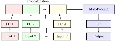
where W = {Wy,z ∣ 0 ≤ y ≤ ∣Y∣, 1 ≤ z ≤ ∣Z∣} is the category weights, and G(X, t) is the feature learner to extract features from X at t. The category weights W includes a set of vectors Wy,z, one for each pair of y and z. The feature learner G(X, t) is a Deep Neural Network (DNN) which yields an effective representation of MTS data. Recall that X is a sequence of d-dim data point, so X can be represented by d channels of univariate time series. The first level of G(X, t) is an input layer. This layer captures a subsequence Xt-w/2∶t+w/2 where w is the window size, and decomposes Xt-w/2∶t+w/2 into d inputs for each channel. The second level of G(X, t) is a group of Fully Connected (FC) layers, where the κ-th FC layer takes the κ-th input and outputs a vector for a channel-independent representation. Then, we concatenate the outputs of those FC layers into one vector using a concatenation layer. Next, we use a Max-Pooling layer to reduce the dimension of the concatenated vector, and then we use a FC layer to extract a feature vector from the pooled vector. This feature vector is the final output of G(X, t). The neural network structure of G(X, t) is illustrated in Figure 1. Given a dataset D = {(X(i) , y(i) , A(i) )}, where A(i) = {a(i) 1 , a(i) 2 , ..., a(i) T (i) } is the ground-truth action sequence corresponding to X(i) , we learn the model p(az ∣ y,X, t ; W,G) in an endto-end fashion as follows:
In the above equation, we jointly maximize three probabilities: (1) p(az = a(i) t,z ∣ 0,X(i) , t ; W,G) is maximized to enhance the weight W0,z regarding the unknown of y; (2) p(az = a(i) t,z ∣ y(i) ,X(i) , t ; W,G) is maximized to enhance the weight Wy(i) ,z regarding y(i) ; (3) p(az = 0 ∣ y′ ,X(i) , t ; W,G) for y′ ∈ Y/{y(i)} are maximized to improve the robustness of the model, since this will force az = 0 when the given y is mistakenly estimated by the CAM during inference. After finding the optimal W ∗ and G∗ , we obtain the model p(A∣ y,X ; θ∗ ) for inferring A, where θ∗ = (W ∗ ,G∗ ).
Complex Activity Model (CAM)
The CAM p(y ∣A; ψ) is used to infer y given A. Let φ(A) be a function that extracts features on the sequence A. We specifically extract the feature of Temporal Patterns [H¨oppner, 2001; Liu et al., 2015], because this feature can effectively capture the temporal relations among actions appearing in arbitrary stages of CAs. Moreover, the Temporal Patterns feature can be represented by a vector of fixed dimension, which enables the training and inference of CAM using action sequences of varied lengths. We propose p(y ∣A; ψ) as follows:
where ψ = {ψy∣1 ≤ y ≤ ∣Y∣} is the weight parameter, and ψ includes a set of vectors ψy as the weights for each y. In the learning procedure of p(y = h ∣A; ψ), we consider that the penalties for the predictions are monotonically increasing with respect to time. This is because that a model should be more certain on the correct prediction when CAs are performed at a later stage [Ma et al., 2016]. Therefore, the CAM can better capture the progressions of CAs with the increasing penalties. Given a dataset D = {(A(i) , y(i) )}, we learn the CAM p(y ∣ A ; ψ) as follows:
where λt is the penalty weight that 0 < λ1 <, ..., < λT (i) ≤ 1. After finding the optimal ψ∗ , we obtain the model p(y ∣A; ψ∗ ) for inferring y.
SimRAD Algorithms
Given the ASM p(A ∣ y, X ; θ) and the CAM p(y ∣ A ; ψ), we introduce the processes of SimRAD to estimate A and y with the two models. SimRAD considers the prediction confidences of the CAs, which are presented by a group of probabilities p0, p1, ..., p∣Y∣ such that ∑∣Y∣ y=0 py = 1. p0 indicates the confidence of that CA is unknown, and py indicates the confidence on y, for 1 ≤ y ≤ ∣Y∣. We initialize p0 = 1, and py = 0 for 1 ≤ y ≤ ∣Y∣. By taking into account the confidences, SimRAD uses the ASM to estimate A by first calculating the probability p(A ∣ X) as:
and then obtain the estimation ˆ A = {ˆa1, ..., ˆan} as:
We present ˆ A as a sequence of estimated action vectors ˆat such that ˆ A = {ˆa1, ..., ˆan}, where ˆat = {ˆat,1, ..., ˆat,∣Z∣}. Let
Algorithm 1 SimRAD Training
Input: A dataset D = {(X(i) , y(i) , A(i) )} Output: The optimal parameters θ∗ and ψ∗ 1: Learn θ = (W,G) using D by Eq. 8 2: Initialize p(i) 0 = 1, p(i) 1 = 0, ..., p(i) ∣Y∣ = 0 for i ∈ {1, ..., ∣D∣} 3: for l = 1, 2, ...,L do 4: Let D′ = ∅ 5: for i = 1, 2, ..., ∣D∣ do 6: Estimate ˆ A(i) using p(i) y s by Eq. 11 and Eq. 12 7: D′ = D′ ⋃{( ˆ A(i) , y(i) )} 8: end for 9: Update ψ using D′ by Eq. 10 10: for i = 1, 2, ..., ∣D∣ do 11: Update p(i) 0 = 1/2, and p(i) y = 1/2 ⋅ p(y ∣ ˆ A(i) ; ψ) for y ∈ Y 12: end for 13: end for 14: return θ∗ = θ, ψ∗ = ψpt,z = p(az = 1 ∣ y,X, t). It can be derived that an ˆat,z of ˆat is given by ˆat,z = 1{∑∣Y∣ y=0 py ⋅pt,z > 0.5}. However, if there is a subset S ⊆ Z such that the actions of S are mutually exclusive and one action must appear, then we obtain ˆ A by setting ˆat,z∗ = 1 where z∗ = argmaxz∈S ∑∣Y∣ y=0 py ⋅ pt,z, and setting ˆat,z = 0 for z ∈ S/{z∗}. With the estimation ˆ A, SimRAD can use the CAM to obtain the estimation ˆ y as:
We then update p0 = 1/2, and py = 1/2 ⋅ p(y ∣ ˆ A;ψ) for 1 ≤ y ≤ ∣Y∣. The p0 is updated to 1/2 as we presume a half confidence on the predictions of the CA. Next, we provide the details of the SimRAD algorithms regarding both training and inferring procedures.
SimRAD Training: Given a training dataset D, we first learn the ASM's parameter θ = (W,G) using D by Eq. 8. Then, we initialize the CAM's parameter ψ and iteratively learn ψ for L rounds. In each round, we use the estimated action sequences instead of ground truth for learning ψ. This makes ψ adapt to θ and achieves desired performance. For an instance (X(i) , y(i) ,A(i) ) ∈ D, we calculate the estimated action sequence ˆ A(i) by Eq. 11 and Eq. 12. Then, the ˆ A(i) s together with y(i) s form a new set of instances D′ , which is used to learn/update ψ. After learning/updating ψ in this round, we can update the p(i) y s for each instance of D. The p(i) y s will be used in the next round for estimating ˆ A(i) . The pseudocode of SimRAD's training algorithm is provided in Algorithm 1. SimRAD Inference: Suppose an ongoing MTS is given by a series of MTS prefixes X1,X2, ...,XT , we predict A and y for T steps. At time t, we calculate the estimated action sequence ˆ At by Eq. 11 and Eq. 12. Then, we update the pys, and obtain the inferred CA by ˆ yt = argmaxy∈Y py. The pseudocode of SimRAD's inference algorithm is provided in Algorithm 2.
Algorithm 2 SimRAD Inference
Input: A series of MTS prefixes X1,X2, ...,XT Output: A series of CA inference outputs ˆ y1, ˆ y2, ..., ˆ yT
- 1: Initialize p0 = 1, p1 = 0, ..., p∣Y∣ = 0
- 2: for t = 1, 2, ...,T do
- 3: Estimate ˆ At using pys by Eq. 11 and Eq. 12
- 4: Update p0 = 1/2, and py = 1/2⋅p(y ∣ ˆ At ; ψ) for y ∈ Y
- 5: ˆ yt = argmaxy∈Y py
- 6: end for
- 7: return ˆ y1, ˆ y2, ..., ˆ yT
4 Experiments
The experiments are conducted on a 64-bit Ubuntu 14.04 LTS operating system. The experimental scripts are written in Python 2.7 with the use of Scikit-learn [Pedregosa et al., 2011] and Keras [Chollet and others, 2015] packages.
Dataset: The experiments are conducted on Opportunity (OPP) dataset [Roggen et al., 2010]. OPP dataset is collected by 4 subjects with sensors placed on their bodies (back, hands, waists, arms, etc), where the sensors' sampling rate is 30 readings per seconds. Each subject is asked to perform 5 complex activities (CAs): relaxing, early morning, coffee time, sandwich time, and cleanup. The relaxing has 40 instances. For the other CAs, each category has 20 instances. The actions appearing in those CAs can be categorized into 3 types: 5 locomotion actions (LocA), 14 left-hand actions (LHA), and 14 right-hand actions (RHA). Each type includes an abnormal action which presents some undefined behaviors, and the other are defined actions, such as 'grabbing'. The actions of each type are mutually exclusive. At any time point, there will be presence of 3 concurrent actions one for each type.
Data Preparation: Although we have only one available CA dataset, the dataset contains a rich amount of data collected by sensors placed on various parts of subjects' body. Therefore, based on OPP dataset, we generate 3 sub-datasets: OPP-BH, OPP-BW, and OPP-BUA for empirical evaluation. Each sub-dataset contains 3 trails of 3-axis accelerations collected by sensors placed on 3 different locations of body. The details of the sensor placement locations of the 3 subdatasets are: 1) OPP-BW: Back, Left Waist, Right Waist; 2) OPP-BH: Back, Left Hand, Right Hand; 3) OPP-BUA: Back, Left Upper Arm, Right Upper Arm. For each sub-dataset, we describe a data instance (X(i) , y(i) ,A(i) ) of D as: X(i) is the multivariate time series (MTS) of the 3 sensors' acceleration data, thereby, the dimension d of each data point x(i) t is 9 (9 channels = 3 sensors × 3 axises); y(i) is the CA label; A(i) is the action sequence, where the dimension of each a(i) t is 33 (33 = 5 LocA + 14 LHA + 14 RHA).
Experimental Settings: We conduct experiments based on 4-fold cross-validation. We consider that the amount of testing data is greater than the training data as CAs can be performed in various individual ways in real-world. Therefore, we use the 1/4 instances regarding one subject for training and the other 3/4 for testing. The evaluation results are reported as the average results of the 4 folds.
Settings of SimRAD: For the action sequence model (ASM), we describe the detailed settings of feature learner G from bottom to top as follows: The input layer uses window size w = 120 for channels of locomotion actions, and uses the half size of w for channels of left/right-hand actions as hand actions are shorter than locomotion actions; The FC layers of each channel output 60-dim vectors; The Max-Pooling layer down-samples the concatenated vector by a scale of 2; The last FC layer outputs a 256-dim vector. We train the ASM with batch size of 10 and training epoch of 50. For the complex activity model (CAM), we set the feature φ(A) as Temporal Patterns of 1-pattern [Liu et al., 2015], and we use quadratic penalty weight λt = (t/T)2 for 1 ≤ t ≤ T. We train SimRAD with learning rounds L = 10. The settings of window size w, penalty weight λt, and learning round L will be studied in subsection 4.1.
Settings of Comparison Methods: We test 5 methods in comparison with SimRAD. The settings of the methods are as following. 1) 1NN+DTW: We use 1-nearest neighbor (1NN) method to classify MTS based on Dynamic Time Wrapping (DTW) distance. 2) 1NN+Fea: For each channel of MTS, we extract AR feature [Kwapisz et al., 2011] and Fourier coefficients of 0Hz, 1Hz, and 2Hz. We combine all these features as a feature vector, and use 1NN to classify the feature vectors based on Euclidean distance. 3) DT+Fea: We extract the same features used in 1NN+Fea, and use decision tree (DT) to classify the feature vectors. 4) LSTM: We implement a Recurrent Neural Network (RNN) based method, where the architecture of the RNN consists of an LSTM layer with 256-dim output, a dense layer with K-dim output, and a softmax layer. 5) MD-MPP: We implement Multilevel-Discretized Marked Point-Process (MD-MPP) based method, where the piece and level parameters are both set to 10 [Li et al., 2014].
4.1 Prediction of Complex Activities
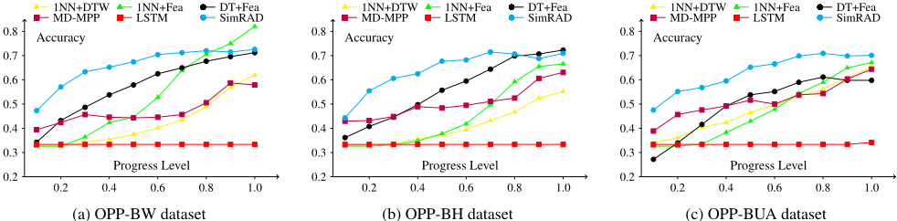
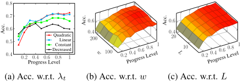
We evaluate the performances of SimRAD and the 5 comparison methods regarding prediction accuracies of CAs at progress levels 0.1, 0.2, ..., 1.0, where the progress level is defined as t/T. According to the evaluation results shown in Figure 2, SimRAD outperforms all the comparison methods in most of the times, except progress levels of 0.9 and 1.0 on OPP-BW and OPP-BH datasets. SimRAD uniformly surpasses the best accuracies of the comparison methods by average 7.2%. It is worth noting that the LSTM based model cannot be effectively learned due to insufficient number of data instances. But LSTM still has a lot potential in the future, when there is a large enough dataset. To statistically compare the performance of SimRAD with the 5 methods, we conduct the Wilcoxon signed-ranked test on the results (40 pairs) of the 3 datasets. The returned R+ and R- correspond to the sum of the ranks of the differences above and below zero, respectively. The returned p-value represents the lowest level of significance of a hypothesis that results in rejection. This value allows one to determine whether two methods have significantly different performances. According to the results shown in Table 1, the p-values in comparisons of SimRAD with all the 5 methods, reject the null hypotheses for accuracy with a level of significant α = 0.0005. Therefore, SimRAD outperforms the 5 comparison methods at all progress levels with high confidence. We study the prediction accuracies of SimRAD with respect to (w.r.t.) penalty weight λt, window size w, and learning round L using the OPP-BW dataset. According to Figure 3a, using penalty weight of Constant λt = 1 or Decreased λt = 1 - t/T obtains slightly better accuracies before 0.3. However, using Linear λt = t/T or Quadratic λt = (t/T)2 obtains surpassing accuracies at later stages. According to Figure 3b, using w between 120 and 150 obtains better accuracies. According to Figure 3c, the accuracies fluctuate a little before L = 10, and then remain stable as L increases beyond 10.
| SimRAD vs. 1NN+DTW | SimRAD vs. 1NN+Fea | SimRAD vs. DT+Fea | SimRAD vs. LSTM | SimRAD vs. MD-MPP | |||||||||||
|---|---|---|---|---|---|---|---|---|---|---|---|---|---|---|---|
| Dataset | R+ | R- | p-value | R+ | R- | p-value | R+ | R- | p-value | R+ | R- | p-value | R+ | R- | p-value |
| OPP-BW | 817.0 | 3.0 | 0.0000 | 720.0 | 100.0 | 0.0000 | 692.0 | 128.0 | 0.0002 | 820.0 | 0.0 | 0.0000 | 761.0 | 59.0 | 0.0000 |
| OPP-BH | 820.0 | 0.0 | 0.0000 | 809.0 | 11.0 | 0.0000 | 738.0 | 82.0 | 0.0000 | 820.0 | 0.0 | 0.0000 | 696.0 | 124.0 | 0.0001 |
| OPP-BUA | 810.0 | 10.0 | 0.0000 | 800.0 | 20.0 | 0.0000 | 769.0 | 51.0 | 0.0000 | 820.0 | 0.0 | 0.0000 | 701.0 | 119.0 | 0.0001 |
4.2 Recognition of Action Sequence
Recall that SimRAD predicts CAs by discovering action sequences from sensor MTS data. We explore the detailed performance of SimRAD by studying the recognition accuracy of the actions. For each time point, we expect to recognize one of 5 LocA, one of 14 LHA, and one of 14 RHA. Therefore, we evaluate the accuracy regarding one action sequence A, where the accuracy is calculated as 1 3n ∑nt=1 (1{LocA correct at t} + 1{LHA correct at t} + 1{RHA correct at t}). We report the averaged accuracies on all the testing X. We compare our ASM with 3 methods: 1) Softmax Regression (SR) with regularization parameter
| Dataset | ASM | SR | LDA | Lasso |
|---|---|---|---|---|
| OPP-BW | 75.06(±12.40) | 35.92(±13.96) | 54.52(±12.55) | 56.86(±13.70) |
| OPP-BH | 73.32(±12.76) | 32.08(±16.03) | 56.23(±11.51) | 59.05(±11.40) |
| OPP-BUA | 74.08(±13.40) | 39.12(±19.62) | 47.12(±18.85) | 57.38(±17.24) |
γ = 0.1; 2) Linear Discriminant Analysis (LDA); 3) Lasso with γ = 0.1. According to the results shown in Table 2, the proposed ASM significantly outperforms the 3 comparison methods. As a result, SimRAD accurately finds the actions for predicting CAs.
5 Conclusion &FutureWork
In this paper, we study the problem of predicting complex activities (CAs) with ongoing multivariate time series (MTS). We propose Simultaneous Complex Activities Recognition and Action Sequence Discovering (SimRAD) which predicts a CA over time by finding a sequence of multivariate actions from sensor MTS data using a Deep Neural Network. SimRAD learns two probabilistic models for inferring CAs and action sequences, where the estimations of the two models are conditionally dependent on each other. SimRAD alternately predicts the CA and the action sequence with the two models, thus the predictions can be mutually updated until the completion of CA. We evaluate SimRAD on a real-world CA dataset of a rich amount of sensor data. The results demonstrate that SimRAD outperforms state-of-the-art methods by average 7.2% in prediction accuracy with very high confidence (p-values < 0.0005).
In future work, we plan to implement SimRAD on mobile platforms, such as smartphones and smartwatches, and test SimRAD in real-time. We will also consider minimizing the computational cost of SimRAD to improve energy-efficiency of the algorithm on mobile devices.
Acknowledgments
This work is supported by Australian Research Council (ARC) Discovery Project DP180102050 and Future Fellowships Project FT120100832.
@inproceedings{ijcai2018p461,
  title     = {Predicting Complex Activities from Ongoing Multivariate Time Series},
  author    = {Cheng, Weihao and Erfani, Sarah and Zhang, Rui and Kotagiri, Ramamohanarao},
  booktitle = {Proceedings of the Twenty-Seventh International Joint Conference on
               Artificial Intelligence, {IJCAI-18}},
  publisher = {International Joint Conferences on Artificial Intelligence Organization},
  editor    = {Jérôme Lang},
  pages     = {3322--3328},
  year      = {2018},
  month     = {7},
  note      = {Main track},
  doi       = {10.24963/ijcai.2018/461},
  url       = {https://doi.org/10.24963/ijcai.2018/461},
}
TY - CPAPER TI - Predicting Complex Activities from Ongoing Multivariate Time Series AU - Cheng, Weihao AU - Erfani, Sarah AU - Zhang, Rui AU - Kotagiri, Ramamohanarao T2 - Proceedings of the Twenty-Seventh International Joint Conference on Artificial Intelligence, IJCAI-18 PB - International Joint Conferences on Artificial Intelligence Organization PY - 2018 SP - 3322 EP - 3328 DO - 10.24963/ijcai.2018/461 UR - https://doi.org/10.24963/ijcai.2018/461 ER -Copied
Machine-readable versions of this paper, for tools and AI agents:





