
NeuCast: Seasonal Neural Forecast of Power Grid Time Series
Proceedings of the Twenty-Seventh International Joint Conference on Artificial Intelligence. Main track. Pages 3315-3321.
https://doi.org/10.24963/ijcai.2018/460
Keywords
- Multidisciplinary Topics and Applications: Multidisciplinary Topics and Applications
- Machine Learning: Time-series;Data Streams
- Machine Learning: Data Mining
Abstract
In the smart power grid, short-term load forecasting (STLF) is a crucial step in scheduling and planning for future load, so as to improve the reliability, cost, and emissions of the power grid. Different from traditional time series forecast, STLF is a more challenging task, because of the complex demand of active and reactive power from numerous categories of electrical loads and the effects of environment. Therefore, we propose NeuCast, a seasonal neural forecasting method, which dynamically models various loads as co-evolving time series in a hidden space, as well as extra weather conditions, in a neural network structure. NeuCast captures seasonality and patterns of the time series by integrating factor modeling and hidden state recognition. NeuCast can also detect anomalies and forecast under different temperature assumptions. Extensive experiments on 134 real-word datasets show the improvements of NeuCast over the stateof-the-art methods.
- [Baliyan et al., 2015] Arjun Baliyan, Kumar Gaurav, and Sudhansu Kumar Mishra. A review of short term load forecasting using artificial neural network models. Pro- cedia Computer Science, 48:121-125, 2015.
- [Box et al., 2015] George E. P. Box, Gwilym M. Jenkins, Gregory C. Reinsel, and Greta M. Ljung. Time series anal- ysis: Forecasting and control, 5th edition. Journal of the Operational Research Society, 22(2):199-201, 2015.
- [Bryan Hooi and Faloutsos, 2018] Amritanshu Pandey Marko Jereminov Larry Pileggi Bryan Hooi, Hyun Ah Song and Christos Faloutsos. Streamcast: Fast and online mining of power grid time sequences. In The 2018 SIAM International Conference on Data Mining, 2018.
- [Daneshi and Daneshi, 2008] H. Daneshi and A. Daneshi. Real time load forecast in power system. In 2008 Third International Conference on Electric Utility Deregulation and Restructuring and Power Technologies, pages 689- 695, 2008.
- [De Livera et al., 2011] Alysha M De Livera, Rob J Hyn- dman, and Ralph D Snyder. Forecasting time series with complex seasonal patterns using exponential smooth- ing. Journal of the American Statistical Association, 106(496):1513-1527, 2011.
- [Dudek, 2016] Grzegorz Dudek. Pattern-based local lin- ear regression models for short-term load forecasting. 130:139-147, 2016.
- [Fan et al., 2016] Guo-Feng Fan, Li-Ling Peng, Wei-Chiang Hong, and Fan Sun. Electric load forecasting by the SVR model with differential empirical mode decomposition and auto regression. 173:958-970, 2016.
- [Ganguly et al., 2017] Piyali Ganguly, Akhtar Kalam, and Aladin Zayegh. Short term load forecasting using fuzzy logic. In International Conference on Research in Educa- tion and Science, 2017.
- [Gers et al., 1999] Felix A Gers, Jürgen Schmidhuber, and Fred Cummins. Learning to forget: Continual prediction with lstm. 1999.
- [Godfrey and Gashler, 2017] Luke B Godfrey and Michael S Gashler. Neural decomposition of time-series data for ef- fective generalization. IEEE transactions on neural net- works and learning systems, 2017.
- [Gross and Galiana, 1987] George Gross and Francisco D Galiana. Short-term load forecasting. Proceedings of the IEEE, 75(12):1558-1573, 1987.
- [He et al., 2017] Xiangnan He, Lizi Liao, Hanwang Zhang, Liqiang Nie, Xia Hu, and Tat-Seng Chua. Neural collabo- rative filtering. pages 173-182. ACM Press, 2017.
- [Jereminov et al., 2017] M Jereminov, A Pandey, HA Song, B Hooi, C Faloutsos, and L Pileggi. Linear load model for robust power system analysis. IEEE PES Innovative Smart Grid Technologies (2017, p.(submitted)) Google Scholar, 2017. [Letchner et al., 2009] Julie Letchner, Christopher Re, Mag- dalena Balazinska, and Matthai Philipose. Access meth- ods for markovian streams. In Data Engineering, 2009. ICDE'09. IEEE 25th International Conference on, pages 246-257. IEEE, 2009.
- [Maas et al., 2013] Andrew L Maas, Awni Y Hannun, and Andrew Y Ng. Rectifier nonlinearities improve neural net- work acoustic models. In Proc. ICML, volume 30, 2013.
- [Matsubara and Sakurai, 2016] Yasuko Matsubara and Ya- sushi Sakurai. Regime shifts in streams: Real-time fore- casting of co-evolving time sequences. In KDD, pages 1045-1054, 2016.
- [Matsubara et al., 2014] Yasuko Matsubara, Yasushi Saku- rai, and Christos Faloutsos. AutoPlait: automatic min- ing of co-evolving time sequences. pages 193-204. ACM Press, 2014.
- [Matsubara et al., 2015] Yasuko Matsubara, Yasushi Saku- rai, and Christos Faloutsos. The web as a jungle: Non- linear dynamical systems for co-evolving online activi- ties. In Proceedings of the 24th International Conference on World Wide Web, pages 721-731. International World Wide Web Conferences Steering Committee, 2015.
- [Salvador and Chan, 2007] Stan Salvador and Philip Chan. Toward accurate dynamic time warping in linear time and space. Intelligent Data Analysis, 11(5):561-580, 2007.
- [Selakov et al., 2014] A Selakov, D Cvijetinović, L Milović, S Mellon, and D Bekut. Hybrid pso-svm method for short- term load forecasting during periods with significant tem- perature variations in city of burbank. Applied Soft Com- puting, 16:80-88, 2014.
- [Shahidehpour et al., 2002] Mohammad Shahidehpour, Ha- tim Yamin, and Zuyi Li. Market Operations in Electric Power Systems, New York, NY: IEEE. Wiley-Interscience, John Wiley & Sons, Inc, 2002.
- [Shen and Li, 2015] Zhushi Shen and Defu Li. Electrici- ty power load yesterday hit a new high to 29.82 mil- lion kilowatts. http://wwww.zhhome.com/news/detail/id- 2930.html, 2015. Link
- [Song et al., 2017] Hyun Ah Song, Bryan Hooi, Marko Jereminov, Amritanshu Pandey, Larry Pileggi, and Chris- tos Faloutsos. PowerCast: Mining and forecasting power grid sequences. In Joint European Conference on Machine Learning and Knowledge Discovery in Databases, pages 606-621. Springer, 2017.
- [Sudheer and Suseelatha, 2015] G Sudheer and A Susee- latha. Short term load forecasting using wavelet transform combined with holt-winters and weighted nearest neigh- bor models. International Journal of Electrical Power & Energy Systems, 64:340-346, 2015.
- [Zheng et al., 2017] Jian Zheng, Cencen Xu, Ziang Zhang, and Xiaohua Li. Electric load forecasting in smart grids using long-short-term-memory based recurrent neural net- work. In Information Sciences and Systems (CISS), 2017 51st Annual Conference on, pages 1-6. IEEE, 2017.
References were extracted automatically from the PDF and may contain errors.
Full text extracted automatically from the PDF; figures, tables and equations may differ. The PDF is the version of record.
1 Introduction
What will the power consumption (including active and reactive power) be at a location of the power grid in the next few days, in face of weather conditions, and numerous resistive and inductive electrical loads, such as heaters, bulbs, air conditioners, and motors? What will the power consumption be if extreme weather occurs, e.g. temperature dramatically increases, or rain/snow comes? These questions are well known as short-term load forecasting (STLF), which is important for guaranteeing a reliable and efficient operation of a power grid system [Daneshi and Daneshi, 2008; Shahidehpour et al., 2002].
Different from general time series, power time series forecasting is more challenging, due to the following characteristics:
1) Complex demand of electrical loads. [Song et al., 2017] tried to use a linear combination of factors related to resistive and inductive loads, to model the dynamics of power demand. Nevertheless, the real situation of various power-factor (ratio of active power) loads makes the modeling of power demand more complex.
* Corresponding Author
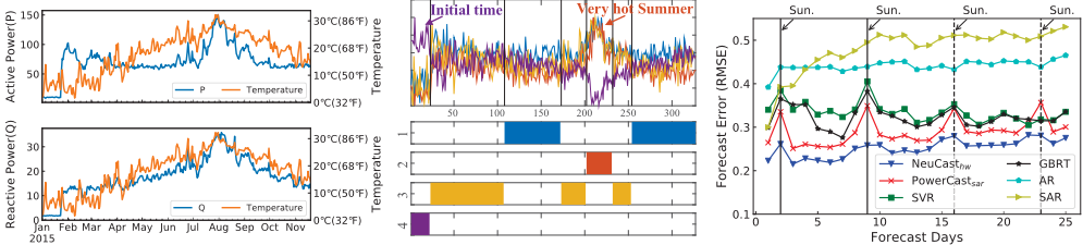
- Seasonality and high-level patterns. Seasonal patterns of power consumption happens in time of day, e.g. rush hours, working hours, and family hours. Existing exponential smoothing [Sudheer and Suseelatha, 2015], and seasonal ARIMA [Box et al., 2015] studied the seasonality in time series. Higher-level patterns are always present as well, such as winter and summer patterns in a year-long observation (see Fig. 1(a)). If those patterns are recognized, we can improve the forecast by 'purifying' the time series using this pattern: meaning, identifying different high-level patterns and filtering the data so as to train using only the relevant pattern. Hidden Markov Models including AutoPlait [Matsubara et al., 2014] and RegimeCast [Matsubara and Sakurai, 2016] can segment and recognize patterns with hidden states. However, the above two groups of related works do not consider both seasonality and such high-level patterns at the same time.
3) External conditions. The increases and decreases of temperature, and precipitation can also affect power consumption. Such conditions can be easily used as features in the feature-based methods [Baliyan et al., 2015; Dudek, 2016]. However, robustness and seasonality cannot be guaranteed in those models.
Therefore, we propose a Neural foreCasting approach, NeuCast, integrating those domain-related characteristics with the time series of a power grid. In NeuCast, a nonlinear deep neural network is designed to model the complex power demand as hidden co-evolving time series, which can be interpreted as different categories of electrical loads. The seasonality is modeled and the high-level patterns are recognized to have a fine-tuned model. We show that NeuCast outperforms the baselines on two real datasets: the dataset of a southern city in China and the CMU dataset. In summary, our main contributions are outlined as follows:
- Novelty of deep forecast framework. We propose a seasonal neural framework for power load forecasting, which models the complex power demand of categories of electrical loads, the seasonality, and high-level pat-
- (a) Power was consumed differently over a year.
- (b) NeuCast identifies high-level patterns for robustness.
- (c) NeuCast keeps the best forecast performance for different lengths.
| AR++ | LR/SVR | ||||
| HMM++ | PowerCast | NeuCast | |||
| Properties | |||||
| Seasonality | ✓ | ✓ | ✓ | ✓ | |
|---|---|---|---|---|---|
| External condition inclusion Modeling complex demand | ✓ | ? | ✓ ✓ | ||
| Pattern discovery | ✓ | ✓ |
Table 1: Comparison between NeuCast and other algorithms.
terns in time series, and external conditions, such as temperature and precipitation.
- Robustness for distinct and anomalous patterns. NeuCast segments and recognizes distinct patterns of time series (see Fig. 1(b)), and filters the data using these patterns, while ignoring anomalous and different patterns for better and robust prediction.
- Effectiveness. NeuCast outputs more accurate forecasts than state-of-the-art methods in 134 real world datasets (see Fig. 1(c)).
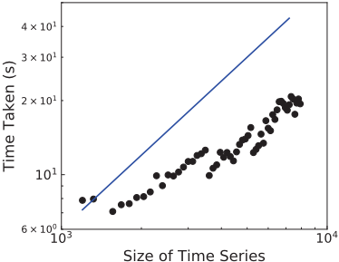
- Scalability. NeuCast is scalable, and runs approximately in linear time of series size.
Reproducibility: Our code is publicly available at https:// github.com/chenpudigege/NeuCast
2 RelatedWork
Time series forecasting has been well studied in past decades. In order to exploit the seasonality in time series, many forecasting methods have been proposed, such as seasonal ARIMA [Box et al., 2015], HoltWinters [Sudheer and Suseelatha, 2015], and TBATS [De Livera et al., 2011]. In order to capture high-level patterns, Hidden Markov Models [Letchner et al., 2009] are employed to segment and recognize highlevel patterns with hidden states to forecast, such as AutoPlait [Matsubara et al., 2014], and Non-linear dynamical systems [Matsubara and Sakurai, 2016; Matsubara et al., 2015]. RNNs including LSTM and GRU were used for STLF task recently as a black-box method [Zheng et al., 2017]. However, RNNs have the weakness for processing long series [Gers et al., 1999], which can be 10 thousand long in power series. RNNs are unable to learn seasonality [Godfrey and Gashler, 2017], since once a forget gate is set, the seasonal history will be lost. Moreover, the anomalous and distinct patterns in a high level may bring noises for prediction.
As a special time series, power grid load forecast has attracted many attention in the past few years. Apart from classical time series approaches, feature-based methods are widely used to capture external factors in power system, such as linear regression (LR) [Dudek, 2016], artificial neural networks (ANNs) [Baliyan et al., 2015] and support vectorregression (SVR) [Selakov et al., 2014; Fan et al., 2016]. Soft computing techniques like fuzzy logic methods [Ganguly et al., 2017] construct a set of logic statements or rules to capture the complex mathematical relationship between features and outputs. Physics-based models [Jereminov et al., 2017; Song et al., 2017; Bryan Hooi and Faloutsos, 2018] used linear combination of active and reactive power consumption to model the dynamics of power demand.
In particular, PowerCast [Song et al., 2017] use latent factor model to capture the seasonality. However, recent research [He et al., 2017] has found that the inner product of traditional latent factor model limit the representation in hidden space. Compared to PowerCast, NeuCast additionally allows for external factors, and uses a non-linear deep neural network to model the complex power consumption with hidden co-evolving time series, as well as identifying high-level patterns to provide better robustness. Table 1 summarizes the well-known time series forecasting methods. Our NeuCast is the only one can handle all the characteristics.
3 The Proposed NeuCast
STLF concerns the future load changes in a short period of time, where the time boundaries may be from the next hour, or possibly half-hour, up to 7 days [Gross and Galiana, 1987]. The definition of STLF problem is as follows:
- Given: historical power grid operation monitoring data, i.e. co-evolving time series X(t) = [x1(t), · · · , xNp (t)],
Algorithm 1 NeuCast Algorithm
Input: Historical observations X(1 : N); External Features E(1 : N +Nf)
Output: X(N : N +Nf)
- 1: Construct X with X(1 : N)
- 2: Construct E with E(1 : N)
- 3: D,H,W, b = random initializing
- 4: D′′ = D
- 5: repeat
- 6: D=D′′
- 7: D,H,W, b = factor modeling by optimizing Eq. (5)
- 8: D′ = [D, ˜D]T , seasonal smoothing to extend D
- 9: D′′ = high-level pattern purification by minimizing Eq. (7)
- 10: until maximum epochs K or D′′ ≡D
- 11: Forecasting X using Eq. (6)
reconstructing the tensor X with extended Nfd days and purification.
3.2 Factor Modeling
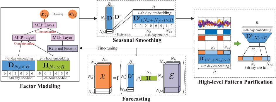
To address the seasonality of the time of day, factor modeling step uses a full neural network to embed the time of day into a shared Nh × R matrix H from input slices of tensor X in the right sub-figure of Fig. 2. It is reasonable because there will be a stronger similarity and temporal dependency between days which have analogous behavior on the hours of the day in the latent space. Moreover, we also learn another day-level factor matrix D. It can be interpreted as the dynamics of different hidden categories of electrical loads every day, e.g. heaters, irons, kettles, and bulbs that only consume active power; and air conditioners and industrial equipments that consume different ratios of reactive power as well.
As the figure shows, the input layer accepts the days and hours with one-hot encoding. The following embedding layers D and H map the sparse representations to dense ones. After getting the embedding vectors of day and hour, we concatenate them to be the input of a fully connected neural net-
where a sequence xp is one type of data e.g. active/reactive power, and t = 1, · · · , N;
- Forecast: the future demand for Nf steps in the future, i.e., X(t), for t = N + 1, · · · , N + Nf .
In the following paper, we use active power and reactive power time series as X(t). Thus we forecast active and reactive power demand for a few hours and days in the future.
3.1 Framework Overview
The overall framework of NeuCast is illustrated in Fig. 2, which is comprised of three key components: factor modeling, seasonal smoothing, and high-level pattern purification. Tensor X ∈ RNd×Nh×Np is reshaped by folding matrix X(t) on date, where Nd is the number of days, Nh = 24 is the number of hours per day, and Np is the number of data types. We forecast Nfd days in the future (i.e., Nf = Nh×Nfd time steps). Tensor E ∈ RNd×Nh×Ne includes external conditions, where Ne is the number of external conditions, e.g. temperature and precipitation. The vector xij and vector eij have Np and Ne elements, by separately slicing X and E on i-th day and j-th hour. Matrix D ∈ RNd×R and matrix H ∈ RNh×R are day-level and hour-level latent matrix learned from the neural networks, where R is the length of a latent vector. Thus we have R co-evolving times series of days represented by D.
As we can see in Alg. 1, to capture external conditions and complex power demand of categories of electrical loads, factor modeling use the non-linear neural networks to factorize various electrical loads as co-evolving time series D and matrix H in a hidden space. Factor modeling also integrates external information by tensor E. Then we proceed with seasonal smoothing to extend D for Nfd days in the future, denoted as D′ . Afterwards, high-level pattern purification step segments and identifies high-level distinct patterns in the time series D′ , which helps to filter out the data with quite distinct patterns or anomalies. With purified D′′ and corresponding day embedding, we fine-tune the factor modeling step until no distinct patterns or anomalies are identified, or reach the max number of iterations. At last, we output the forecast by work, i.e. MLP (Multi-Layer Perceptron). Simultaneously, the external information such as temperature and precipitation values are binned as vectors and fed into another MLP unit. Afterwards, in the upper-level MLP unit, the outputs of two MLP units separately from day and hour embedding, and external information are concatenated as a new input. At the end, the prediction of ˆxij for the given date and hour is the output from upper-level MLP.
The overall formula in factor modeling are as follows.
where oDi and oHj denotes the one-hot encoding of i-th day and j-th hour. ˆxij denotes the output vector of power demand of different types. eij is external feature vector of the given date i and hour j. The parameters that need to be optimized include D, H and the parameters on the edges of neural network in MLP units. We then define functions φ and ϕ for two types of MLP units.
where Wl, bl, and al denote the weight matrix, bias vector, and activation function for the l-th layer's perceptron, while ⊕ denotes the concatenation of two vectors. Here, we use the leaky rectified linear function (LReL) [Maas et al., 2013] as the activation function to avoid the dead relu problem at hidden layers and output layer. Finally, the model can be expressed as
where φMF , ϕEXT and φFU are the functions of the three MLP units in Fig. 2 respectively.
The model can be trained by minimizing mean squared error between the predicted value ˆxij and the truth xij:
where λ and ω are the regularization coefficients.
3.3 Seasonal Smoothing and Forecasting
Seasonal smoothing are used for extending the Nfd days of co-evolving time series D for prediction.
We apply an alternative smoothing method on columns of matrix D for extending Nfd more rows as the middle upper part of Fig. 2 shows. Smoothing methods like Seasonal ARIMA and Holt-Winters can incorporate the given time series D, and capture seasonality in day-level. Here, we set the periodicity parameter to be 7 for smoothing to capture the weekly seasonality. As a result, D′ = [D, ˜D]T, where ˜D is the extended Nfd rows.
In the forecast step, we feed extended ˜D into the neural network to forecast the power demand of all types.
where ˜ di is the i-th row of ˜D, and hj is the j-th row of H.
However, before forecasting, we can purify D′ with highlevel patterns, and fine-tune the neural network for better prediction, which is introduced in the following section.
3.4 High-level Pattern Purification
NeuCast uses high-level pattern purification to segment coevolving time series and identify the non-seasonal distinct patters, e.g. 1) daily demand between summer and autumn in one year-long data; 2) anomalies such as equipment debugging and sensor failures. NeuCast uses AutoPlait method to solve the following segmentation and pattern identification problem:
- determine the number of segments m in extended coevolving sequence D′ , and their positions, i.e. S = {s1, ..., sm}, where a segment si represents a day interval;
- determine the number of high-level patterns (regimes) r for those m segments, and the membership of each segment, i.e., F = {f1, ..., fm};
- estimate the model parameters of the r regimes, i.e. Θ = {θ1, ..., θr, Δr×r}, where θi denotes the HMM parameters of the i-th regime, and δij ∈ Δ is the transition probability from the i-th regime to the j-th regime.
To solve the problem, AutoPlait uses MDL (minimum description length) principle as model cost Cost(D′ ;C) to choose among alternative solutions of segmentation and patterns. C is an alternative solution. InMDL, all the parameters and solutions are needed to be encoded, and find a solution minimizing the coding length. The total cost Cost(D′ ;C) includes three parts: CostA, the coding length of segmentation and pattern assignment; CostM(Θ), the coding length for describing model parameters of Θ; and CostC(D′ |Θ), the negative log-likelihood of co-evolving sequence D′ given Θ. AutoPlait sums those three parts up with equal weights in total cost. But we need a discount coefficient to tune the granularity of the distinct patterns (regimes), because if the granularity is too large, NeuCast cannot identify distinct patterns or anomalies; if there are too many small regimes, NeuCast may not get sufficient data for fine-tuning factor modeling. Therefore, we use a hyper-parameter α to discount the cost of parameter coding length CostM(Θ) for regimes:
In such a way, we can give more discount to the cost of parameters describing regimes, in order to encourage to identify more distinct patterns, and vice versa. We will show the effects of α in the experiments.
Afterwards, let the forecasting part of time series, i.e. D′Nd+1···Nd+Nfd , be in a regime τ ∈ [r]. We keep a subset of segments S ′ ⊆ S, which si ∈ S ′ if fi = τ, i = 1, · · · ,m. In other words, we filter out all distinct segments. Besides, if the forecasting part belongs to more than one patterns, we simply use the first one since the forecasting accuracy of the first day is more important. As a result, a purified day-level embedding D′′ is obtained by masking with S ′ . Finally, D′′ is fed to factor modeling for fine tuning.
| SC data | CMU data | |
|---|---|---|
| # of time series (locations) | 133 | 1 |
| # of days | 328 | 23 |
| # of daily samples | 24 | 24 |
| size of each time series | 7872 | 552 |
| monitoring types | [P, Q] | [Ir, Ii, Vr, Vi] |
4 Experiments
We design the experiments to answer the following questions:
- Q1. Forecasting accuracy: how accurately does NeuCast forecast on real-world power grid time series? How does it perform when predicting more days in the future?
- Q2. Anomalous-pattern awareness: how does NeuCast forecast if a time series contains anomalous patterns or distinct patterns?
- Q3. Scalability: how does the algorithm scale with the data size?
We use a one-year-long data and 23-day-long data in Table 2, both from the real-world power grid systems, to evaluate our methods. As the table shows, we collect data from 133 locations in the power grid of a southern city in China (SC data), from Jan. 1 to Nov. 24 in 2015. The other one is a publicly available data from Carnegie Mellon University (CMU), which is 23-day long from Jul. 29 to Aug. 20 in 2016.
In order to use the PowerCast model, we convert the monitoring active/reactive powers: P(t) and Q(t) in the Threephase AC to active/reactive currents: Ir(t) and Ii(t), and voltages: Vr(t) and Vi(t). The conversion equations are shown as follows:
where V denotes line voltage which is a constant, i.e. V = 10(kV).
4.1 Q1. Forecasting Accuracy
Baselines. We use the following baselines:
- auto-regressions: ARIMA (AR) and seasonal ARIMA (SAR), where parameters are chosen using AIC (Akaike information criterion).
- feature-based regressions: Support Vector Regression (SVR), and Gradient Boosted Regression Tree (GBRT). We extract temporal features including hour and weekday with one-hot encoding, and external features of temperature and precipitation. RBF kernel is used for SVR, and penalty for the error term is set to 1. We use 100 trees in GBRT to fit data, and the learning rate is 0.1.
- PowerCast: PowerCastar and PowerCastsar [Song et al., 2017]. We use the parameter settings suggested by the paper.
Experimental setup. We conduct our experiments on a server with NVIDIA GeForce GTX1080×2, and implement NeuCast based on Keras. In the neural network, the latent vector size is 4, and each MLP unit has one hidden layer with 16 neurons. In the training, the batch size is 32, and learning rate is 0.0005. A hyper parameter α in high-level distinct pattern recognition [Matsubara et al., 2014] decides how many distinct patterns we should identify. With validation on the time series data, we found that when α = 0.2, we can get stable and better forecast accuracy. And we set the number of maximum epoch K=2. NeuCast is also implemented with different smoothing methods: ARIMA denoted as NeuCastar, seasonal ARIMA as NeuCastsar, and Holt-Winters denoted as NeuCasthw. NeuCast with and without high-level pattern purification, are separately denoted as NeuCast and NeuCast-.
We use the following forecast error metrics for evaluation, which smaller error indicates better accuracy.
DTW: a widely used distance measure in time series [Salvador and Chan, 2007];
Results. We compare the forecasting performance on 133 different locations of SC data, and the average results and significance value are reported in Table 3. We use 323-daylong time series in each location for training, and forecast the next 5 days. We can see that our NeuCasthw achieves the smallest forecast errors, with stringent significance level (p-value < 0.01). Generally, factorization-based methods, i.e. PowerCast and our NeuCast performs better than those auto-regression and feature-based regression models, since they make effort to model the power demand of categories of electrical loads with hidden co-evolving time series. Moreover, all the configurations of NeuCast have a better forecast. NeuCast with high-level pattern purification can filter out the anomalous data and distinct patterns, and achieves better results than NeuCast-, which guarantees the robustness of our NeuCast in face of anomalies. Especially, NeuCasthw improves the recent state-of-the-art method PowerCast by a range of roughly 18% to 26% in different metrics. Thus we can achieve more accurate forecasts in a year-long SC data using our NeuCast approach.
| Methods | DTW | RMSE | MAE | SMAPE |
|---|---|---|---|---|
| AR | 7.500∗ | 0.4166∗ | 9.321∗ | 0.4803∗ |
| SAR | 6.509∗ | 0.3954∗ | 8.659∗ | 0.5175∗ |
| SVR | 5.116∗ | 0.3114∗ | 7.160∗ | 0.4203∗ |
| GBRT | 4.868∗ | 0.3044∗ | 6.827∗ | 0.3770∗ |
| PowerCastar | 4.294∗ | 0.2729∗ | 6.041∗ | 0.3765∗ |
| PowerCastsar | 4.070∗ | 0.2590∗ | 5.686∗ | 0.3632∗ |
| NeuCast-ar | 3.288 | 0.2338 | 4.669 | 0.2868 |
| NeuCastar | 3.210 | 0.2307 | 4.568 | 0.2831 |
| NeuCast-sar | 3.191 | 0.2275 | 4.557 | 0.2840 |
| NeuCastsar | 3.123 | 0.2238 | 4.429 | 0.2793 |
| NeuCast-hw | 3.089 | 0.2198 | 4.363 | 0.2805 |
| NeuCasthw | 2.972 | 0.2120 | 4.170 | 0.2706 |
| Improvement | 26.9% | 18.1% | 26.6% | 25.4% |
| Methods | DTW | RMSE | MAE | SMAPE |
|---|---|---|---|---|
| AR | 17.22 | 0.08181 | 21.03 | 0.05967 |
| SAR | 17.06 | 0.08187 | 20.78 | 0.05891 |
| SVR | 8.274 | 0.05701 | 15.05 | 0.04661 |
| GBRT | 7.468 | 0.06094 | 15.36 | 0.04614 |
| PowerCastar | 6.834 | 0.05033 | 12.68 | 0.04011 |
| PowerCastsar | 6.887 | 0.05039 | 12.72 | 0.04016 |
| NeuCast-ar | 6.418 | 0.04945 | 11.92 | 0.03686 |
| NeuCast-sar | 6.515 | 0.04999 | 12.18 | 0.03763 |
| NeuCast-hw | 9.263 | 0.06229 | 17.83 | 0.05551 |
| Improvement | 6.08% | 1.74% | 5.99% | 8.10% |
We also test our NeuCast on the public CMU data, and the results of forecasting the last 5 days are reported in Table 4. Since CMU data is 23-days long, we use the data of the first 18 days for training. We forecast active and reactive currents using our NeuCast, and run 10 times training and average testing results to reduce randomness of neural model. Since only one high-level pattern can be identified in such a short time series, NeuCast- and NeuCast achieve the same results. The result of NeuCast- is only reported in the table. As we can see, NeuCast- also achieves the best results. The table shows that NeuCast-ar with ARIMA outperforms NeuCast-hw with Holt-Winters, because Holt-Winters as a triple exponential smoothing method may lead to overfitting on such short time series.
Moreover, when comparing to PowerCast with NeuCast using the same smoothing function, NeuCast-ar and NeuCast-sar have a smaller error in all of the metrics, indicating that the neural network captures more information than the linear factorization.
Finally, we also compare NeuCast with others on forecasting the next 25 days for each location in SC data. The results are illustrated in Fig. 1(c). The RMSE results are averaged over 133 locations for each day. The figure shows that our NeuCast keeps slow growth of forecast errors, which gives a robust and stable results, and outperforms the baselines. The weekday and weekend features are given to SVR, GBRT, and NeuCast. Even though NeuCast has relatively small fluctuations on weekend forecast, it is interesting to see that the forecast of all the methods fluctuates on weekends, which may show more complicated behaviors of people and the demand of electrical loads on weekends than regular work days.
4.2 Q2. Anomalous-pattern Awareness
The Fig. 1 (b) shows the results that we can identify anomalous patterns and distinct patterns in a time series of location #9 in SC data. The patterns around Jan and Aug are quite different from other time in the hidden co-evolving time series.
As we confirmed with the system operators, they initialized the system around Jan (see Fig. 1(a)), and it was a very hot summer in Aug of that year [Shen and Li, 2015]. Thus with the purification, we can filter out those anomalous patterns for better and robust prediction.
4.3 Q3. Scalability
To test the efficiency of NeuCast, we train NeuCast with different size of time series in SC data. The total time consumed by training and forecasting is plotted in black solid dots in Fig. 3. The blue line is a linear relation in log-scale axes. The horizontal axis is the size of training time series. The figure shows that the trend of the scattering points is almost parallel to the blue line, which indicates linear running time in the size of training time series.
5 Conclusion and FutureWork
We propose a neural forecast approach, NeuCast, to forecast time series of a power grid. NeuCast takes complex power demand, seasonality and high-level patterns in time series, and external conditions into consideration. NeuCast outputs more accurate results than the state-of-the-art methods in 134 real world datasets.
For future work, we will try to apply NeuCast to other similar domains, e.g. traffic flow forecast, and computation cluster load forecast. Moreover, additional information, such as geo-locations and connections between the stations will be studied to improve the forecast accuracy.
Acknowledgments
This work is supported in part by the National Hightech R&D Program (No. 2015AA050203) and the National Grand Fundamental Research 973 Program of China (No.2014CB340401). This work is also supported in part by the National Natural Science Foundation of China (No. 61772082, 61772498, 61375058), and the Beijing Municipal Natural Science Foundation (4182043, 4172059).
@inproceedings{ijcai2018p460,
  title     = {NeuCast: Seasonal Neural Forecast of Power Grid Time Series},
  author    = {Chen, Pudi and Liu, Shenghua and Shi, Chuan and Hooi, Bryan and Wang, Bai and Cheng, Xueqi},
  booktitle = {Proceedings of the Twenty-Seventh International Joint Conference on
               Artificial Intelligence, {IJCAI-18}},
  publisher = {International Joint Conferences on Artificial Intelligence Organization},
  editor    = {Jérôme Lang},
  pages     = {3315--3321},
  year      = {2018},
  month     = {7},
  note      = {Main track},
  doi       = {10.24963/ijcai.2018/460},
  url       = {https://doi.org/10.24963/ijcai.2018/460},
}
TY - CPAPER TI - NeuCast: Seasonal Neural Forecast of Power Grid Time Series AU - Chen, Pudi AU - Liu, Shenghua AU - Shi, Chuan AU - Hooi, Bryan AU - Wang, Bai AU - Cheng, Xueqi T2 - Proceedings of the Twenty-Seventh International Joint Conference on Artificial Intelligence, IJCAI-18 PB - International Joint Conferences on Artificial Intelligence Organization PY - 2018 SP - 3315 EP - 3321 DO - 10.24963/ijcai.2018/460 UR - https://doi.org/10.24963/ijcai.2018/460 ER -Copied
Machine-readable versions of this paper, for tools and AI agents:





