
Beyond Similar and Dissimilar Relations : A Kernel Regression Formulation for Metric Learning
Proceedings of the Twenty-Seventh International Joint Conference on Artificial Intelligence. Main track. Pages 3242-3248.
https://doi.org/10.24963/ijcai.2018/450
Keywords
- Machine Learning: Multi-instance;Multi-label;Multi-view learning
- Machine Learning: Dimensionality Reduction and Manifold Learning
- Machine Learning: Classification
Abstract
Most existing metric learning methods focus on learning a similarity or distance measure relying on similar and dissimilar relations between sample pairs. However, pairs of samples cannot be simply identified as similar or dissimilar in many real-world applications, e.g., multi-label learning, label distribution learning or tasks with continuous decision values. To this end, in this paper we propose a novel relation alignment metric learning (RAML) formulation to handle the metric learning problem in those scenarios. Since the relation of two samples can be measured by the difference degree of the decision values, motivated by the consistency of the sample relations in the feature space and decision space, our proposed RAML utilizes the sample relations in the decision space to guide the metric learning in the feature space. Specifically, our RAML method formulates metric learning as a kernel regression problem, which can be efficiently optimized by the standard regression solvers. We carry out several experiments on the single-label classification, multi-label classification, and label distribution learning tasks, to demonstrate that our method achieves favorable performance against the state-of-the-art methods.
- [Bhadra et al., 2017] Sahely Bhadra, Samuel Kaski, and Juho Rousu. Multi-view kernel completion. Machine Learning, 106(5):713-739, 2017.
- [Bhatia et al., 2015] Kush Bhatia, Himanshu Jain, Purushot- tam Kar, Manik Varma, and Prateek Jain. Sparse local em- beddings for extreme multi-label classification. In NIPS, pages 730-738, 2015.
- [Boutell et al., 2004] Matthew R Boutell, Jiebo Luo, Xipeng Shen, and Christopher M Brown. Learning multi-label scene classification. Pattern recognition, 37(9):1757- 1771, 2004.
- [Cha, 2007] Sung-Hyuk Cha. Comprehensive survey on distance/similarity measures between probability density functions. City, 1(2):1, 2007.
- [Cortes et al., 2012] Corinna Cortes, Mehryar Mohri, and Afshin Rostamizadeh. Algorithms for learning kernels based on centered alignment. Journal of Machine Learn- ing Research, 13(Mar):795-828, 2012.
- [Davis et al., 2007] Jason V Davis, Brian Kulis, Prateek Jain, Suvrit Sra, and Inderjit S Dhillon. Information-theoretic metric learning. In ICML, pages 209-216, 2007.
- [Drucker et al., 1997] Harris Drucker, Christopher J. C. Burges, Linda Kaufman, Alex J. Smola, and Vladimir Vapnik. Support vector regression machines. NIPS, 28(7):779-784, 1997.
- [Geng, 2016] Xin Geng. Label distribution learning. IEEE TKDE, 28(7):1734-1748, 2016.
- [Gu et al., 2016] Yuwen Gu, Hui Zou, et al. High- dimensional generalizations of asymmetric least squares regression and their applications. The Annals of Statistics, 44(6):2661-2694, 2016.
- [Guillaumin et al., 2009] Matthieu Guillaumin, Jakob Ver- beek, and Cordelia Schmid. Is that you? metric learning approaches for face identification. In ICCV, pages 498- 505. IEEE, 2009.
- [Hoi et al., 2006] Steven CH Hoi, Wei Liu, Michael R Lyu, and Wei-Ying Ma. Learning distance metrics with contex- tual constraints for image retrieval. In CVPR, volume 2, pages 2072-2078, 2006.
- [Law et al., 2013] Marc T Law, Nicolas Thome, and Matthieu Cord. Quadruplet-wise image similarity learn- ing. In ICCV, pages 249-256, 2013.
- [Li et al., 2012] Zhen Li, Liangliang Cao, Shiyu Chang, John R Smith, and Thomas S Huang. Beyond mahalanobis distance: Learning second-order discriminant function for people verification. In CVPRW, pages 45-50. IEEE, 2012.
- [Liao et al., 2015] Shengcai Liao, Yang Hu, Xiangyu Zhu, and Stan Z Li. Person re-identification by local maximal occurrence representation and metric learning. In CVPR, pages 2197-2206, 2015.
- [McFee and Lanckriet, 2011] Brian McFee and Gert Lanck- riet. Learning multi-modal similarity. Journal of machine learning research, 12(Feb):491-523, 2011.
- [Mensink et al., 2012] Thomas Mensink, Jakob Verbeek, Florent Perronnin, and Gabriela Csurka. Metric learning for large scale image classification: Generalizing to new classes at near-zero cost. ECCV, pages 488-501, 2012.
- [Mu et al., 2010] Yadong Mu, Jialie Shen, and Shuicheng Yan. Weakly-supervised hashing in kernel space. In CVPR, pages 3344-3351. IEEE, 2010.
- [Oh Song et al., 2016] Hyun Oh Song, Yu Xiang, Stefanie Jegelka, and Silvio Savarese. Deep metric learning via lift- ed structured feature embedding. In CVPR, pages 4004- 4012, 2016.
- [Shaw et al., 2011] Blake Shaw, Bert Huang, and Tony Je- bara. Learning a distance metric from a network. In NIPS, pages 1899-1907, 2011.
- [Trohidis et al., 2008] Konstantinos Trohidis, Grigorios T- soumakas, George Kalliris, and Ioannis P Vlahavas. Multi- label classification of music into emotions. In ISMIR, vol- ume 8, pages 325-330, 2008.
- [Wang et al., 2015] Faqiang Wang, Wangmeng Zuo, Lei Zhang, Deyu Meng, and David Zhang. A kernel clas- sification framework for metric learning. IEEE TNNLS, 26(9):1950-1962, 2015.
- [Wang et al., 2016] Kaiye Wang, Ran He, Liang Wang, Wei Wang, and Tieniu Tan. Joint feature selection and sub- space learning for cross-modal retrieval. IEEE TPAMI, 38(10):2010-2023, 2016.
- [Weinberger and Saul, 2009] Kilian Q Weinberger and Lawrence K Saul. Distance metric learning for large mar- gin nearest neighbor classification. Journal of Machine Learning Research, 10(Feb):207-244, 2009.
- [Yang et al., 2006] Liu Yang, Rong Jin, Rahul Sukthankar, and Yi Liu. An efficient algorithm for local distance metric learning. In AAAI, volume 2, pages 543-548, 2006.
- [Ying and Li, 2012] Yiming Ying and Peng Li. Distance metric learning with eigenvalue optimization. Journal of Machine Learning Research, 13(Jan):1-26, 2012.
- [Zadeh et al., 2016] Pourya Zadeh, Reshad Hosseini, and Suvrit Sra. Geometric mean metric learning. In ICML, pages 2464-2471, 2016.
- [Zhang and Wu, 2015] Min-Ling Zhang and Lei Wu. Lift: Multi-label learning with label-specific features. IEEE T- PAMI, 37(1):107-120, 2015.
- [Zhang and Zhou, 2007] Min-Ling Zhang and Zhi-Hua Zhou. Ml-knn: A lazy learning approach to multi-label learning. Pattern recognition, 40(7):2038-2048, 2007.
References were extracted automatically from the PDF and may contain errors.
Full text extracted automatically from the PDF; figures, tables and equations may differ. The PDF is the version of record.
1 Introduction
In many computer vision and pattern recognition tasks, e.g., face recognition [Guillaumin et al., 2009], image classification [Mensink et al., 2012], and person re-identification [Liao et al., 2015], it is crucial to learn a discriminative distance metric to measure the similarity between pairs of samples. Intuitively, metric learning aims to learn a discriminative similarity or dissimilarity metric by pushing the dissimilar samples away and pulling the similar samples together. Typical distance metrics include Euclidean distance, cosine distance, and Mahalanobis distance. Most existing metric learning methods focus on learning a discriminative Mahalanobis distance. Beyond Mahalanobis distance, generalized distance metric learning methods are presented by learning high-order discriminant functions [Li et al., 2012].
∗The corresponding author
According to the availability of the label information, metric learning can be partitioned into three categories, i.e., the unsupervised, semi-supervised and supervised methods. To deal with the heterogeneous data, multi-modal [McFee and Lanckriet, 2011] and cross-modal [Wang et al., 2016] metric learning algorithms are developed. Because of the diversity of the feature space, linear, kernel and tensor distance metrics are learned for different data structures. Different from shallow metric learning, deep learning based methods learn the feature and metric jointly and achieve superior performance [Oh Song et al., 2016].
One of the key steps in existing metric learning methods is to generate doublet [Davis et al., 2007], triplet [Weinberger and Saul, 2009] or even quadruplet [Law et al., 2013] constraints using the label information. Doublet constraints are the most commonly used in metric learning methods. Similar and dissimilar sample pairs are generated in the k-nearest neighbors or ε-neighborhood by measuring whether two samples belong to the same class. In some applications, e.g., weakly supervised learning [Mu et al., 2010] or social networks [Shaw et al., 2011], sample pairs are generated from connectivity information or other side information. Generally, there are two sets of sample pairs, i.e., one contains the similar sample pairs and the other one contains the dissimilar ones.
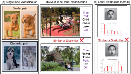
However, for some learning tasks, e.g., multi-label learning [Zhang and Wu, 2015] and label distribution learning [Geng, 2016], relations between sample pairs cannot be simply identified as similar or dissimilar. Thus, the existing metric learning methods cannot work on the above tasks. As shown in Figure 1(a), for single-label classification, it is very simple to identify two images as similar or dissimilar. Figure 1(b) shows there are two scene images that share part of the labels (tree, park, and girl). The problem arises that it is difficult to classify two images into similar or dissimilar sample pair. Figure 1(c) is an example of label distribution learning, where decision space is modeled by label distributions rather than discrete labels. Above discussions encourage us to propose a generalized metric learning method, which can be flexibly adopted to various kinds of tasks.
In machine learning community, one of the basic assumptions is that samples should keep with the same relations in different spaces, especially in the feature space and label space. The principle of metric learning is to encourage samples in the feature space to satisfy the expected relations induced by supervised information. Manifold learning emphasizes locality preserving, which requires that the nearest neighbors of samples should be close to each other in the projected low-dimensional feature space [Yang et al., 2006]. For kernel learning machines, the kernel matrix can be considered as the similarity relation of all samples. Kernel alignment exploits the similarity between kernel matrices for learning kernels [Cortes et al., 2012] and matrix completion [Bhadra et al., 2017]. For multi-modal learning, the sample relation in feature spaces of different modalities should be consistent with that in the label space. For metric learning, as long as the sample relations in the decision space are modeled, the distance metric can be learned by minimizing the difference between sample relations in feature space and decision space.
In this paper, we propose a metric learning formulation, namely relation alignment metric learning (RAML). Our RAML aims to restrain that sample relations measured by metric in the feature space tend to be consistent with those in the decision space during learning. The contributions of this paper are summarized as follows.
- A novel metric learning formulation is proposed to learn distance metrics for different learning tasks, including single-label learning, multi-label learning, and label distribution learning.
- The proposed RAML is formulated as a kernel regression model. Based on RAML formulation, two metric learning methods are developed, i.e., support vector regression metric learning and ridge regression metric learning. Furthermore, we analyze the generalization error bound for the proposed metric learning methods.
- Experiments on single-label classification, multi-label classification and label distribution learning tasks show that our RAML method achieves superior performance against the state-of-the-art methods.
2 Problem Statement
Most existing metric learning methods focus on learning the Mahalanobis distance. Given two samples xi and xj, where xi ∈ Rd and d is the dimension of the feature space, the Mahalanobis distance between the two samples xi and xj, is defined as
where M ∈ Rd×d is a positive semi-definite (PSD) matrix. The parameter M can be predefined, i.e., the inverse of the covariance matrix, or learned by distance metric learning methods.
Generally, metric learning enlarges the distances between dissimilar samples while reduces the distances between similar ones. Two samples with the same label form a positive pair, and ones with the different labels form a negative pair. In supervised learning, sample pairs are previously given in [Guillaumin et al., 2009] or generated based on the available label information [Weinberger and Saul, 2009]. However, in some applications, e.g., multi-label learning, and label distribution learning tasks, two samples cannot be simply classified as positive or negative ones. Let y = [y1, ..., yk, ..., yc] be the label vector of x. For the traditional single-label classification task, x can only belong to one class. If x belongs to the k-th class, yk = 1; otherwise, yk = 0. Different from the traditional single-label classification task, multi-label classification assumes that x can belong to multiple classes. For label distribution learning, there are two constraints for y, i.e., yk ≥ 0, k = 1, 2, ...c, and ∑ck=1 yk = 1. Different from the existing metric learning methods only designed for traditional single-label classification task, we aims at designing a novel metric learning formulation to accommodate different learning tasks.
3 AKernel Regression Formulation
In this section, we present a kernel regression formulation for metric learning. Different from the existing metric learning methods, this method can be used for various kinds of tasks.
3.1 Relation Alignment Learning
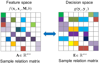
For metric learning, doublet constraint is a kind of description of relationship between a pair of samples in the decision space. As shown in Figure 2, f(xi, xj,M, b) is used to measure the sample relations in feature space while g(yi, yj) is used to measure the sample relations in decision space. g(yi, yj) is specially designed for different tasks. Let A ∈ Rn×n and E ∈ Rn×n be the sample relation matrix in feature and decision spaces, respectively. In general, sample relation in the feature space should be consistent with that in the decision space, i.e.,
where aij and eij represent the sample relation of xi and xj in the feature space and decision space, respectively. Here, to keep consistency, we require that
where g(yi, yj) is the difference degree of two samples in the decision space. g(yi, yj) reflects the sample relation in the decision space, and guides the learning of (M, b) in feature space.
where 〈·, ·〉 is defined as the Frobenius inner product of two matrices, b is the bias item, and Tij = (xi - xj) (xi - xj)T . Then we rewrite (2) to
Once the relation function g(yi, yj) is chosen, (4) can be considered as a linear regression problem. Hence, the metric learning problem is converted to solve a sample pair regression problem with the scaled second sample moment Tij of sample pair (xi, xj) as the input.
3.2 Sample Pair Kernel
To formulate the sample pair regression problem in (4), we introduce a 2-degree polynomial kernel for sample pairs. Let zi denote the sample pair (xi1, xi2). Then the 2-degree polynomial kernel is defined as
With the sample pair kernel, given a sample pair z = (x1, x2), the regression function can be rewritten as
where T = (x1 -x2) (x1 -x2)T and Ti = (xi1 -xi2) (xi1 -xi2)T . Here M = ∑ni=1 βiTi. M is actually a linear combination of the scaled sample moments of the difference between two samples in one pair.
3.3 RegressionMetric Learning
We aim to learn the discriminative M for Mahalanobis distance with a kernel regression formulation, then our Relation Alignment Metric Learning (RAML) can be formulated as
where r(M) is the regularization item imposed on M, λ is a positive constant and l(M, zi, g(zi)) is the regression loss function. The parameter M is learned using (7) for enhancing the consistency of the sample relation in the feature space and decision space. The combinations of different regularization on M and loss functions will lead to different metric learning models. In this paper, we investigate two widely used regression models, i.e., support vector regression (SVR) [Drucker et al., 1997] and ridge regression [Gu et al., 2016].
4 Support Vector RegressionMetric Learning
We first extend our RAML formulation (7) to develop a SVRlike distance metric method:
where ξi and ξ ∗ i are slack variables, and ρ(ξ, ξ ∗ ) is the margin loss item. If we adopt the Frobenius norm to regularize M and ε-sensitive loss function, then this is a standard SVR model. We can also choose other regularizer and loss functions, e.g., sparse regularizer, the Laplacian loss function or the Huberis loss function. As there are a lot of large-scale and efficient SVR solvers, we tend to develop a SVR-like model. Additionally, the variants of SVR have been well investigated, including semi-supervised SVR and multi-kernel SVR. Therefore, the proposed model can be used for semisupervised metric learning, multi-modal metric learning and other specific learning tasks.
In this section, we will discuss how to learn the distance metric via support vector regression. By using Frobenius norm regularization for r(M) and ε-sensitive loss function for ρ(ξ, ξ ∗ ), the metric learning problem in (8) can be formulated as:
where ‖M‖2F is the Frobenius norm of M, and λ is a trade-off constant. By using the Lagrange multipliers, we have
Algorithm 1 The algorithms of our proposed RAML-SVR and RAML-KRR
Input:
Training data X ∈ Rd×m, where d and m are the numbers of feature dimension and samples, respectively.
- 1: Generate sample pairs (xi1, xi2),i = 1, 2, ..., n.
- 2: Compute sample relation g(xi1, xi2),i = 1, 2, ..., n.
- 3: RAML-SVR: Solve (9) by SVR solvers
RAML-KRR: Solve (17) by (20)
- 4: RAML-SVR: M= ∑ni=1 (ai -a∗i )Ti. RAML-KRR: M = ∑ni=1 βiTi .
Output:
Distance metric matrix M
All dual variables should satisfy the positivity constraints, i.e., ai, a∗i , ηi, η∗ i ≥ 0. According to the saddle point condition, the partial derivatives of L with respect to the primal variables will be vanishing, i.e.,
Substituting (11), (12) and (13) into (10), we get the dual optimization problem of (9) with
Similar to the solution of SVR, we can get the solution for (14), i.e.,
Then, the corresponding regression function can be rewritten as
For the metric learning task, M is required to be positive semi-definite. Whereas, the solution for (14) cannot ensure that M is a PSD matrix. We compute the singular value decomposition of M = UΛV and only keep the positive part of Λ to form a new matrix Λ+. Finally, we obtain the PSD matrix M = UΛ+V. The corresponding metric learning (RAML-SVR) algorithm is summarized in Algorithm 1.
5 Ridge RegressionMetric Learning
Besides support vector regression, we also incorporate kernel ridge regression into our RAML formulation (7) for metric learning. As M = ∑ni=1 βiTi, it is equivalent to regularize M by regularizing β. The metric learning problem in (7) can be formulated as:
where f(zj) = ∑ni=1 βi 〈Tj,Ti〉 + b, and r (β) is the regularization item for β . When l2-norm regularization is imposed on β, the objective function becomes
By setting the partial derivatives of L with respect to the variable β to 0, we have
Furthermore, with β we can compute M = ∑ni=1 βiTi. The corresponding metric learning (RAML-KRR) algorithm is summarized in Algorithm 1.
6 Discussion
6.1 Generalization Error Analysis
Let P be a fixed (but unknown) distribution over X×Y. Let each training point (xi, yi)ϵD be sampled i.i.d. from P. Metric learning aims to learn a discriminative matrix M which can preserve the sample relations in the label space. Then metric learning can be formulated as the following stochastic optimization problem:
In fact, (7) minimizes a regularized empirical estimation of (21), i.e., regularized Empirical Risk Minimization (ERM) w.r.t. (21). Following the theoretical analysis in [Bhatia et al., 2015], using techniques from the AUC maximization literature, the excess risk bound for the problem in (7) is given as follows:
Theorem 1. Assume that all data points are confined to a ball of radius R, i.e., ‖x‖2 ≤ R for all x ∈ X. With probability at least 1-δ over the sampling of the dataset D, the solution ˆM to the optimization problem (7) satisfies
where ˆM is the minimizer of (7), v = Lλ and M :={M∈ Rd×d : M⪰ 0}. ¯L is the average number of labels active in a data point.
We can see(22) shows that the optimal solution ˆM to (7) minimizes (21) with an additive approximation error. Additionally, the generalization error bound is independent of the feature dimension.
| Data | S/F/C | ITML LDML | LMNN | DSVM GMML | DML | RAML-SVR RAML-KRR |
|---|---|---|---|---|---|---|
| iris | 150/5/3 | 0.9400±0.0668 0.9633±0.0562 | 0.9528±0.0843 | 0.9400±0.0584 0.9467±0.0689 | 0.9667±0.0471 | 0.9667±0.0423 0.9667±0.0471 |
| wpbc | 198/34/2 | 0.6919±0.0886 0.7629±0.0819 | 0.7432±0.1052 | 0.7329±0.0555 0.6968±0.0714 | 0.7476±0.0776 | 0.7632±0.0608 0.7879±0.0520 |
| wine | 178/14/3 | 0.9607±0.0300 0.9833±0.0268 | 0.9722±0.0393 | 0.9611±0.0375 0.9604±0.0379 | 0.9764±0.0425 | 0.9667±0.0468 0.9833±0.0268 |
| sonar | 208/61/2 | 0.8558±0.0615 0.7638±0.0903 | 0.8462±0.0705 | 0.8657±0.0583 0.8560±0.0749 | 0.8369±0.0840 | 0.8900±0.0591 0.8850±0.0454 |
| glass | 214/10/6 | 0.6636±0.0997 0.5740±0.1266 | 0.6556±0.0797 | 0.6258±0.1109 0.6308±0.1100 | 0.5724±0.1032 | 0.6735±0.1072 0.6395±0.1040 |
| wdbc | 569/31/2 | 0.9666±0.0263 0.9685±0.0284 | 0.9719±0.0223 | 0.9561±0.0355 0.9631±0.0315 | 0.9631±0.0193 | 0.9789±0.0162 0.9755±0.0237 |
| credit | 690/15/2 | 0.8043±0.0496 0.8422±0.0517 | 0.8436±0.0525 | 0.8013±0.0540 0.7941±0.0508 | 0.8261±0.0531 | 0.8246±0.0461 0.8479±0.0320 |
| Data | S/F/C ITML | LDML LMNN | DSVM | GMML | DML | RAML-SVR | RAML-KRR |
|---|---|---|---|---|---|---|---|
| binalpha | 1404/320/36 0.6303±0.0501 | 0.6542±0.0317 0.6112±0.0358 | 0.5625±0.0322 | 0.5338±0.1986 | 0.5063±0.0251 | 0.7250±0.0348 | 0.6850±0.0351 |
| caltech101 | 8641/256/101 0.5803±0.0162 | 0.5528±0.0157 0.5795±0.0126 | 0.5584±0.0159 | 0.5500±0.0117 | 0.3936±0.0123 | 0.5855±0.0095 | 0.5803±0.0147 |
| MnistDat | 3495/784/10 0.8695±0.0142 | 0.8858±0.0124 0.8721±0.0255 | 0.8848±0.0194 | 0.8589±0.0171 | 0.8323±0.0239 | 0.9019±0.0175 | 0.9087±0.0137 |
| Mpeg7 | 1400/6000/70 0.8214±0.0333 | 0.7971±0.0365 0.8253±0.0232 | 0.8271±0.0353 | 0.8429±0.0228 | 0.7071±0.0267 | 0.8450±0.0305 | 0.7936±0.0341 |
| MSRA25 | 1799/256/12 0.9989±0.0168 | 0.9978±0.0046 | 0.9923±0.0397 0.9950±0.0121 | 0.9956±0.0140 | 0.9817±0.0211 | 0.9989±0.0023 | 0.9980±0.0142 |
| news20 | 3970/8014/4 0.8678±0.0200 | 0.8816±0.0145 | 0.8734±0.0290 0.8594±0.0159 | 0.8647±0.0143 | 0.8166±0.0222 | 0.9025±0.0132 | 0.9217±0.0145 |
| TDT2 20 | 1938/3677/20 0.9587±0.0358 | 0.9531±0.0306 | 0.9352±0.0197 0.9499±0.0175 | 0.9437±0.0275 | 0.6333±0.0176 | 0.9679±0.0244 | 0.9762±0.0164 |
| uspst | 2007/256/10 0.8979±0.0261 | 0.9084±0.0243 | 0.9096±0.0217 0.9125±0.0172 | 0.8858±0.0168 | 0.8030±0.0330 | 0.9525±0.0147 | 0.9447±0.0157 |
7 Experiments
In this section, we conduct experiments to validate the performance of the proposed metric learning methods. We consider three applications, including single-label classification, multi-label classification and label distribution learning. The following part will be organized as the corresponding three parts.
7.1 Single-Label Classification
Experiment setup. We first verify the effectiveness of RAML on seven UCI datasets 1 and eight image datasets 2 . The detailed information of these datasets is listed in Table ?? and Table ??, where "S/F/C" represents the number of samples, features and classes. We compare RAML with the stateof-the-art methods, i.e., ITML [Davis et al., 2007], LMNN [Weinberger and Saul, 2009], DML [Ying and Li, 2012], DoubletSVM (DSVM) [Wang et al., 2015], GMML [Zadeh et al., 2016] on each dataset. For fair comparison, the parameters of all compared methods are set as the default setting of the original references. For DSVM, we set k = 1, and the penalty factor C < 10, 000. For GMML, the weight t is set within [0,1] and chosen by greedy search. Ten-fold cross validation is introduced to evaluate the metric learning performance, i.e., 90% for training and 10% for testing. The average accuracy of 10-fold cross validation is reported.
Experimental analysis. Table ?? and Table ?? list the classification accuracy of different metric learning methods on UCI datasets and image datasets, respectively, where the best results are marked in bold face. RAML-SVR and RAML-KRR indicate support vector regression metric learning and ridge regression metric learning, respectively. RAML achieves superior results in terms of the evaluation criteria on most dataset. The performance of RAML-SVR is similar to RAML-KRR. For RAML-KRR, when the number of samples increase significantly, the efficiency will be reduced because
1 http://archive.ics.uci.edu/ml/index.php
2 http://www.escience.cn/people/fpnie/index.html
6.2 Sample Relation Function
The motivation of RAML is keeping relation consistency in different spaces, including feature space and label space. As the sample relations in the decision space are used to guide the metric learning in feature space, it is important to choose proper sample relation functions for different kinds of decision spaces. We consider three learning tasks, i.e., single label learning, multi-label learning and label distribution learning. Let yi and yj denote the label vector of xi and xj. The sample relation function is defined as:
where ‖a‖1 is the l1-norm of a. For single label classification, when g(yi, yj) is defined as (23), RAML degenerates to a sample pair classification problem. For multi-label learning, (23) reflects the difference with respect to positive classes of two samples. For label distribution learning, there are many metrics to evaluate the difference between two distributions. Here, we experimentally find that (23) reflects sample difference in the decision space and achieves superior performance. Therefore, we choose (23) for all the three learning tasks. The choice of optimal relation functions for different tasks are still an open problem, which will be investigated in our future work. If we want to learn a similarity metric in feature space, the inner product of two vectors, or other kernel functions can be used for g(yi, yj).
6.3 Sample Pair Selection
Relation alignment learning aims to preserve the consistency of the sample relations between the feature space and the decision space. However, we do not need to use the relations of all sample pairs. For support vector regression, the support vectors are mainly lying on the decision boundary. Therefore, sample pairs are only generated in the k nearest neighbors (default value of k is 3 for our method RAML), which is similar to most existing metric learning algorithms. Besides, using only part of sample pairs can greatly reduce computational complexity and storage burden.
its time complexity is o(n3 ), where n is the number of samples.
7.2 Multi-Label Classification
Datasets. In this section, we evaluate the proposed method using three datasets 3 , i.e., emotion [Trohidis et al., 2008], flags, and corel800 dataset [Hoi et al., 2006]. The emotion dataset [Trohidis et al., 2008] consists of 100 songs from each of the following 7 different genres, Classical, Reggae, Rock, Pop, Hip-Hop, Techno and Jazz. The collection was created from 233 musical albums choosing three songs from each album. The flag dataset contains 194 instances, 19 features and 7 labels (red, green, blue, yellow, white, black, orange). The corel 800 dataset [Hoi et al., 2006] contains 800 grayscale images of 10 individuals with 80 images per class.
Evaluation metrics. We employ five multi-label classification measures as evaluation metrics including Hamming loss, ranking loss, one error, coverage and average precision. Hamming loss measures accuracy in a multi-label classification task. Ranking loss has the property that the minimization of the loss functions will lead to the maximization of the ranking measures. MLKNN is the multi-label version of KNN [Zhang and Zhou, 2007] and it is based on statistical information derived from the label sets of an unseen instance's neighboring instances. As no specific metric learning algorithms are developed for MLKNN, here we use MLKNN as the baseline. If the performance of RAML is superior to MLKNN, the effectiveness of RAML is verified.
Experimental analysis. Experimental results of RAML and MLKNN are reported in Table 3, where the best result on each evaluation criterion is shown in bold face. The "↓" after the measures indicates "the smaller the better" and "↑" after the measures indicates "the larger the better". As shown in Table 3, both RAML-SVR and RAML-KRR achieve superior results in terms of the five evaluation measures. Compared with MLKNN, RAML can learn a discriminative distance metric, making the sample relation in the feature space more consistent with that in the decision space.
| Data | emotion | flags | corel800 | |
|---|---|---|---|---|
| MLKNN | Hamming Loss↓ | 0.2137 | 0.3099 | 0.0137 |
| Ranking Loss↓ | 0.1729 | 0.2228 | 0.1888 | |
| One Error↓ | 0.3317 | 0.2154 | 0.6825 | |
| Coverage↓ | 1.9158 | 3.8154 | 88.5100 | |
| Average Precision↑ | 0.7808 | 0.8084 | 0.3276 | |
| RAML-SVR | Hamming Loss↓ | 0.2054 | 0.2967 | 0.0135 |
| Ranking Loss↓ | 0.1577 | 0.2179 | 0.1882 | |
| One Error↓ | 0.2376 | 0.2000 | 0.6425 | |
| Coverage↓ | 1.8960 | 3.8115 | 88.2350 | |
| Average Precision↑ | 0.8101 | 0.8128 | 0.3386 | |
| RAML-KRR | Hamming Loss↓ | 0.2046 | 0.2967 | 0.0134 |
| Ranking Loss↓ | 0.1382 | 0.2113 | 0.1888 | |
| One Error↓ | 0.2574 | 0.2000 | 0.6550 | |
| Coverage↓ | 1.7327 | 3.7692 | 88.5100 | |
| Average Precision↑ | 0.8225 | 0.8112 | 0.3388 |
3 http://mulan.sourceforge.net/datasets-mlc.html
7.3 Label Distribution Learning
Datasets. The dataset employed in this experiment includes 2,000 natural scene images [Zhang and Zhou, 2007]. There are nine possible labels associated with these images, i.e., plant, sky, cloud, snow, building, desert, mountain, water and sun. The image features are extracted using the method in [Boutell et al., 2004]. Each image is represented by a feature vector of 294 dimensions. The output of each instance is a distribution rather than discrete labels. AAKNN is the extended version of KNN in label distribution learning. Here AAKNN is used as the baseline without metric learning in the label distribution task.
Evaluation metrics. Different from both the single label output and the label set output of multi-label learning, the output of label distribution learning algorithm is a label distribution. The evaluation measures for label distribution learning is the average distance or similarity between the predicted and real label distributions. On a particular dataset, each of the measures may reflect some aspects of an algorithm. It is hard to say which evaluation metric is the best. Therefore, we use several measures to evaluate the proposed algorithm, and compare RAML with the classical AAKNN method. Finally we employ five measures: Chebyshev distance (Cheb), Clark distance (Clark), Canberra metric (Canber), cosine coefficient (Cosine), and intersection similarity(Intersec) [Cha, 2007]. The first three are distance measures and the last two are similarity measures.
Experimental analysis. Table 4 shows RAML and AAKNN in terms of five measures. We show the best result with respect to each measure in bold face. The "↓" after the measures indicates "the smaller the better". "↑" after the measures indicates "the larger the better". One can easily conclude that our RAML methods perform better than AAKNN in terms of five different measures. It owes to more discriminative metric learned by the proposed RAML formulation.
| Criterion | AAKNN | RAML-SVR | RAML-KRR |
|---|---|---|---|
| Chebyshev↓ | 0.3261±0.0120 | 0.3102±0.0123 | 0.3139±0.0157 |
| Clark↓ | 1.8448±0.0233 | 1.6986±0.0386 | 1.6865±0.0468 |
| Canberra↓ | 4.3412±0.0650 | 3.8576±0.1316 | 3.8419±0.1316 |
| Cosine↑ | 0.6905±0.0167 | 0.7051±0.0167 | 0.7057±0.0126 |
| Intersection↑ | 0.5506±0.0120 | 0.5739±0.0261 | 0.5743±0.0172 |
8 Conclusions
In this paper, we proposed a relation alignment metric learning (RAML) formulation to learn distance metrics for various kinds of learning tasks. Different from all existing methods relying on similar and dissimilar relations between sample pairs, we formulated metric learning problem as a kernel regression model via relation alignment learning. Based on our RAML formulation, two metric learning methods are instantiated with support vector regression and kernel ridge regression. Experimental result show RAML is very competitive with state-of-the-art metric learning methods on single-label classification, moreover it can improve the performance of multi-label learning and label distribution learning tasks.
Acknowledgments
This work was supported by the National Natural Science Foundation of China under Grants 61502332 and 61732011, Natural Science Foundation of Tianjin Under Grants 17JCZDJC30800.
@inproceedings{ijcai2018p450,
  title     = {Beyond Similar and Dissimilar Relations : A Kernel Regression Formulation for Metric Learning},
  author    = {Zhu, Pengfei and Qi, Ren and Hu, Qinghua and Wang, Qilong and Zhang, Changqing and Yang, Liu},
  booktitle = {Proceedings of the Twenty-Seventh International Joint Conference on
               Artificial Intelligence, {IJCAI-18}},
  publisher = {International Joint Conferences on Artificial Intelligence Organization},
  editor    = {Jérôme Lang},
  pages     = {3242--3248},
  year      = {2018},
  month     = {7},
  note      = {Main track},
  doi       = {10.24963/ijcai.2018/450},
  url       = {https://doi.org/10.24963/ijcai.2018/450},
}
TY - CPAPER TI - Beyond Similar and Dissimilar Relations : A Kernel Regression Formulation for Metric Learning AU - Zhu, Pengfei AU - Qi, Ren AU - Hu, Qinghua AU - Wang, Qilong AU - Zhang, Changqing AU - Yang, Liu T2 - Proceedings of the Twenty-Seventh International Joint Conference on Artificial Intelligence, IJCAI-18 PB - International Joint Conferences on Artificial Intelligence Organization PY - 2018 SP - 3242 EP - 3248 DO - 10.24963/ijcai.2018/450 UR - https://doi.org/10.24963/ijcai.2018/450 ER -Copied
Machine-readable versions of this paper, for tools and AI agents:





