
Where to Prune: Using LSTM to Guide End-to-end Pruning
Proceedings of the Twenty-Seventh International Joint Conference on Artificial Intelligence. Main track. Pages 3205-3211.
https://doi.org/10.24963/ijcai.2018/445
Keywords
- Machine Learning: Deep Learning
- Computer Vision: Computer Vision
- Machine Learning: Reinforcement Learning
Abstract
Recent years have witnessed the great success of convolutional neural networks (CNNs) in many related fields. However, its huge model size and computation complexity bring in difficulty when deploying CNNs in some scenarios, like embedded system with low computation power. To address this issue, many works have been proposed to prune filters in CNNs to reduce computation. However, they mainly focus on seeking which filters are unimportant in a layer and then prune filters layer by layer or globally. In this paper, we argue that the pruning order is also very significant for model pruning. We propose a novel approach to figure out which layers should be pruned in each step. First, we utilize a long short-term memory (LSTM) to learn the hierarchical characteristics of a network and generate a pruning decision for each layer, which is the main difference from previous works. Next, a channel-based method is adopted to evaluate the importance of filters in a to-be-pruned layer, followed by an accelerated recovery step. Experimental results demonstrate that our approach is capable of reducing 70.1% FLOPs for VGG and 47.5% for Resnet-56 with comparable accuracy. Also, the learning results seem to reveal the sensitivity of each network layer.
- [Ba and Caruana, 2014] Jimmy Ba and Rich Caruana. Do deep nets really need to be deep? In Advances in neural information processing systems, pages 2654-2662, 2014.
- [Baker et al., 2016] Bowen Baker, Otkrist Gupta, Nikhil Naik, and Ramesh Raskar. Designing neural network ar- chitectures using reinforcement learning. In ICLR, 2016.
- [Cun et al., 1990] Yann Le Cun, John S. Denker, and Sara A. Solla. Optimal brain damage. In Advances in neural in- formation processing systems, volume 2, pages 598-605, 1990.
- [Denton et al., 2014] Emily L Denton, Wojciech Zaremba, Joan Bruna, Yann LeCun, and Rob Fergus. Exploiting linear structure within convolutional networks for efficient evaluation. In Advances in neural information processing systems, pages 1269-1277, 2014.
- [Girshick, 2015] Ross Girshick. Fast r-cnn. In ICCV, pages 1440-1448, 2015.
- [Han et al., 2016] Song Han, Huizi Mao, and William J Dally. Deep compression: Compressing deep neural net- works with pruning, trained quantization and huffman cod- ing. In ICLR, 2016.
- [Hassibi and Stork, 1993] Babak Hassibi and David G Stork. Second order derivatives for network pruning: Optimal brain surgeon. In Advances in neural information process- ing systems, pages 164-171, 1993.
- [He et al., 2015] Kaiming He, Xiangyu Zhang, Shaoqing Ren, and Jian Sun. Delving deep into rectifiers: Surpass- ing human-level performance on imagenet classification. In ICCV, 2015.
- [He et al., 2016] Kaiming He, Xiangyu Zhang, Shaoqing Ren, and Jian Sun. Deep residual learning for image recog- nition. In CVPR, pages 770-778, 2016.
- [Hochreiter and Schmidhuber, 1997] Sepp Hochreiter and Jürgen Schmidhuber. Long short-term memory. Neural computation, 9(8):1735-1780, 1997.
- [Hu et al., 2016] Hengyuan Hu, Rui Peng, Yu-Wing Tai, and Chi-Keung Tang. Network trimming: A data-driven neu- ron pruning approach towards efficient deep architectures. arXiv preprint arXiv:1607.03250, 2016.
- [Ioffe and Szegedy, 2015] Sergey Ioffe and Christian Szegedy. Batch normalization: Accelerating deep net- work training by reducing internal covariate shift. In ICML, pages 448-456, 2015.
- [Krizhevsky and Hinton, 2009] Alex Krizhevsky and Geof- frey Hinton. Learning multiple layers of features from tiny images. Tech Report, 2009.
- [Krizhevsky et al., 2012] Alex Krizhevsky, Ilya Sutskever, and Geoffrey E Hinton. Imagenet classification with deep convolutional neural networks. In Advances in neural in- formation processing systems, pages 1097-1105, 2012.
- [LeCun et al., 1990] Yann LeCun, Bernhard E Boser, John S Denker, Donnie Henderson, Richard E Howard, Wayne E Hubbard, and Lawrence D Jackel. Handwritten digit recognition with a back-propagation network. In Advances in neural information processing systems, pages 396-404, 1990.
- [Li et al., 2017] Hao Li, Asim Kadav, Igor Durdanovic, Hanan Samet, and Hans Peter Graf. Pruning filters for efficient convnets. In ICLR, 2017.
- [Liu et al., 2017] Zhuang Liu, Jianguo Li, Zhiqiang Shen, Gao Huang, Shoumeng Yan, and Changshui Zhang. Learning efficient convolutional networks through net- work slimming. arXiv preprint arXiv:1708.06519, 2017.
- [Luo et al., 2017] Jian-Hao Luo, Jianxin Wu, and Weiyao Lin. Thinet: A filter level pruning method for deep neural network compression. arXiv preprint arXiv:1707.06342, 2017.
- [Molchanov et al., 2017] Pavlo Molchanov, Stephen Tyree, Tero Karras, Timo Aila, and Jan Kautz. Pruning convolu- tional neural networks for resource efficient transfer learn- ing. In ICLR, 2017.
- [Rastegari et al., 2016] Mohammad Rastegari, Vicente Or- donez, Joseph Redmon, and Ali Farhadi. Xnor-net: Ima- genet classification using binary convolutional neural net- works. In ECCV, pages 525-542. Springer, 2016.
- [Scardapane et al., 2017] Simone Scardapane, Danilo Com- miniello, Amir Hussain, and Aurelio Uncini. Group sparse regularization for deep neural networks. Neurocomputing, 2017.
- [Schroff et al., 2015] Florian Schroff, Dmitry Kalenichenko, and James Philbin. Facenet: A unified embedding for face recognition and clustering. In CVPR, pages 815-823, 2015.
- [Simonyan and Zisserman, 2015] Karen Simonyan and An- drew Zisserman. Very deep convolutional networks for large-scale image recognition. In ICLR, 2015.
- [Wen et al., 2016] Wei Wen, Chunpeng Wu, Yandan Wang, Yiran Chen, and Hai Li. Learning structured sparsity in deep neural networks. In Advances in neural information processing systems, pages 2074-2082, 2016.
- [Williams, 1992] Ronald J Williams. Simple statistical gradient-following algorithms for connectionist reinforce- ment learning. Machine learning, 8(3-4):229-256, 1992.
- [Xie and Yuille, 2017] Lingxi Xie and Alan Yuille. Genetic cnn. arXiv preprint arXiv:1703.01513, 2017.
- [Zhang et al., 2017] Xuan Zhang, Hao Luo, Xing Fan, Weilai Xiang, Yixiao Sun, Qiqi Xiao, Wei Jiang, Chi Zhang, and Jian Sun. Alignedreid: Surpassing human- level performance in person re-identification. arXiv preprint arXiv:1711.08184, 2017.
- [Zoph and Le, 2017] Barret Zoph and Quoc V Le. Neural architecture search with reinforcement learning. In ICLR, 2017.
- [Zoph et al., 2017] Barret Zoph, Vijay Vasudevan, Jonathon Shlens, and Quoc V Le. Learning transferable archi- tectures for scalable image recognition. arXiv preprint arXiv:1707.07012, 2017.
References were extracted automatically from the PDF and may contain errors.
Full text extracted automatically from the PDF; figures, tables and equations may differ. The PDF is the version of record.
1 Introduction
Deep convolutional neural networks (CNNs) have achieved impressive results in many computer vision tasks, like image classification [Simonyan and Zisserman, 2015; He et al., 2016], object detection [Girshick, 2015], and face recognization [Schroff et al., 2015]. Starting from simple architectures like LeNet [LeCun et al., 1990], researchers have proposed more complicated and powerful architectures, such as AlexNet [Krizhevsky et al., 2012], VGG [Simonyan and Zisserman, 2015], and ResNet [He et al., 2016], which progressively lead to better performance. In some cases, CNNs are even capable of surpassing human-level performanc [He et al., 2015; Zhang et al., 2017; Schroff et al., 2015]. Owing to the promising results, CNNs have attracted considerable attention from the academia and the industry.
∗This work was supported by the National Natural Science Foundation of China (No. 61571269). Corresponding authors: Guiguang Ding and Bin Wang.
Apart from the accuracy, the model complexity of CNNs is also an important issue, especially in real-world applications, because it is very often that we have to run deep model on cheap devices with limited computation resources and lowfrequency CPUs, like a mobile phone. In this case, it is desired that the CNNs are tiny and fast enough while preserving the accuracy. To address this issue, deep model compression techniques have become a popular research topic.
Generally speaking, model compression techniques fall into four categories. The first category is quantization. In [Rastegari et al., 2016], a model binarization approach is proposed. Although significant speed-up has been achieved, binarized network suffers from performance drop and less robustness. The second category is sparseness [Cun et al., 1990; Hassibi and Stork, 1993] by removing unimportant weights (or setting it to zero). Unfortunately, the sparse matrix calculation cannot be accelerated by the existing software and hardware libraries at present. The third category is tensor factorization [Denton et al., 2014] which uses a combination of smaller tensors and simpler operations to approximate larger tensors and complicated operations. Although it may lead to smaller and faster networks, it degrades the performance, especially for complicated tasks. The fourth category is filter-level pruning [Li et al., 2017; Molchanov et al., 2017] which directly removes unimportant convolutional kernels. Pruning can well preserve the structure of the network, which leads to smaller and faster models with little or no performance drop and seems simpler compared to the previous techniques. Because of these advantages, pruning has drawn the most attention in recent years, which is the main focus of this paper.
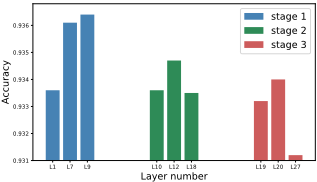
Intuitively, deep model compression is a systematical task which should utilize the whole model to make decisions for pruning. However, it seems that most existing pruning approaches [Li et al., 2017; Hu et al., 2016; Luo et al., 2017; Liu et al., 2017] only consider local information. In particular, they mostly focus on evaluating the importance of each filter individually in each layer and prune filters layer by layer sequentially from top to bottom or bottom to top. At each step, some filters are pruned in a layer, and the next layer is processed in the next step. However, an essential phenomenon is ignored that the layers are different in terms of the importance. If it happens to prune a few filters of an important layer, the performance of the overall systemmay significantly drop. On the other hand, pruning many filters in an unimportant layer may have little influence on accuracy but significantly reduce model complexity. To demonstrate this, we take ResNet-56 as an example. We remove the same number of filters in different layers in a stage so that the complexities after pruning are identical. The experiments in each stage are independent. We show the accuracy of the model after pruning different layers (e.g., L10, L12, or L18 in stage 2) in Figure 1. Obviously, different layers have different importance, so they have the observable different impact on the whole system. Therefore, where to prune is a critical issue for pruning and choosing the right layer may end up more complexity reduction and less performance drop. In Table 3, we report the comparison between an orderly pruning method [Li et al., 2017] and the proposed pruning approach with layer selection. We can observe that our approach achieves larger pruning rate with comparable accuracy.
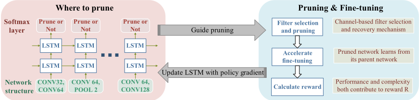
The above phenomenon motivates us to investigate the problem of choosing the right layer to prune in each step. In this paper, we propose a novel approach to evaluate the importance of each layer and choose less important layers to prune. In particular, considering that a CNN is a hierarchical structure and can be represented as a string, we employ long short-term memory (LSTM) [Hochreiter and Schmidhuber, 1997] as an evaluation model to generate the pruning decision for each layer, which is capable of finding the most unimportant layers first. The LSTM is trained in a reinforcement learning way with model performance and complexity as the reward. Then a channel-based method is adopted to evaluate the importance of each filter in the chosen layer, and some unimportant filters are pruned combined with the recovery mechanism. With several pruning steps, the complexity achieves the required level while little or no performance drop is accomplished. The complete framework is shown in Figure 2, and our major contributions are summarized as follows:
- We argue and demonstrate that where to prune is a critical issue at each step and we introduce an end-to-end framework to prune models in the correct order.
- Considering the hierarchical structure of CNNs, we employ LSTM as an evaluation model to find the most unimportant layer and generate the pruning decision.
- Our end-to-end method is capable of compressing a variety of network structures largely with comparable accuracy and works well on both convolutional and fullyconnected networks.
- The experimental results reveal that our method learns the sensitivity of each network layer well.
2 RelatedWork
Our work is in relation to model pruning, network structure search, and some other issues, each being elaborated below.
2.1 Pruning
Removing network connections is an intuitive model compression method, which mostly focuses on evaluating and selecting unimportant connections. [Hassibi and Stork, 1993] assess the network connections by the second-order derivative information, but it results in high computational complexity. [Han et al., 2016] compress models in three steps: removing connections with smallest absolute weights values, quantization, and Huffman encoding. [Scardapane et al., 2017; Wen et al., 2016] regularize neural network parameters by group Lasso penalty leading to sparsity on a group level.
The above methods introduce sparsity in the parameter tensors which is difficult to be accelerated by existing software and hardware libraries. In order to achieve accelerated performance, more works focus on filter-wise pruning which could preserve the network structure well. [Li et al., 2017] assess the importance of a filter by calculating its absolute weights sum and remove unimportant filters layer by layer. [Hu et al., 2016] observe that filters with more zero activation neurons are redundant. [Molchanov et al., 2017] evaluate filters by estimating their effect on the cost function through Taylor expansion and prune the less important filters under a global threshold. Recently, [Luo et al., 2017] consider filter pruning as an optimization problem and prunes filters based on its next layer. However, its greedy algorithm of selecting filters based on the overall loss is computationally complex. [Liu et al., 2017] leverage the scaling factors in batchnorm layers to evaluate filters combining with sparsity regularization.
Most of the existing methods prune filters layer by layer, or they globally prune all unimportant filters simultaneously. However, they do not take importance level of each layer into account. In other words, a proper algorithm should selectively prune layers in terms of their contributions to the whole model. Existing algorithms pay more attention to evaluating filters but not giving a reasonable pruning order. We suggest selecting the most unimportant layers first and then evaluating the importance of each filter in the chosen layers to prune.
2.2 Network Structure Search
Current widely used network structures are designed manually based on expert knowledge. These networks fit some datasets well, but they are not optimal for diversified data in the real world. In order to release human labor and produce optimal networks, two mainstream methods based on reinforcement learning and genetic algorithm are proposed respectively. [Zoph and Le, 2017; Baker et al., 2016] use the recurrent neural network(RNN) to generate complete network descriptions from scratch, and the RNN is trained by a reinforcement learning method. As a network architecture can be described as a string, [Xie and Yuille, 2017] define some genetic operations: selection, mutation, and crossover to produce new network structures from generation to generation. However, due to the huge network search space, methods above consume enormous time and hardware resources. Inspired by that, [Zoph et al., 2017] search for an architectural building block on a small dataset and then transfer the block to a larger dataset.
2.3 OtherWorks
Besides compressing big networks, there is another way of training mall networks directly. [Ba and Caruana, 2014] observe that if a small network can learn the essence of condensed knowledge, it will have similar performance to the big networks. They propose a distillation method that one or more big networks are taken as teacher networks and a small network as the student network to learn teachers' predictive distributions. By minimizing the squared error between the two logits produced by the teachers and student, the student's performance approximates to the teachers'.
3 Method
In this section, we give a detailed introduction to our end-toend pruning method. Firstly, we introduce how LSTM generates pruning strategies and how reinforcement learning helps to train LSTM in Section 3.1. Next, our filter selection strategy and accelerated training skills are presented in Section
- The end-to-end pruning framework in Figure. 2 is illustrated as follows.
- (a). Pruning guidance. An initial or intermediate network representation is fed into LSTM, and LSTM generates a strategy which layers should be pruned.
- (b). Filter selection and pruning. We evaluate the importance of each filter in the layers chosen by LSTM with a channel-based method, then prune those unimportant filters combined with the recovery mechanism.
- (c). Accelerating fine-tuning. The pruned model is finetuned to restore its performance. We utilize the distillation method to accelerate the fine-tuning process.
- (d). Updating LSTM. We update LSTM in a reinforcement learning way with both performance and complexity of the pruned model as the reward signal.
- (e). Repeat from (a) to (e).
3.1 Where to Prune
Input and Output of LSTM
A neural network is a hierarchical sequence from input to output connected by operation nodes. These nodes can be convolution, pooling and fully-connected operation. For a common CNN here, the ith node ξi is denoted as (mi, ni), where operation type m is in {0, 1, 2} corresponding to convolution, pooling, and fully-connected block respectively, operation attribute n equals to filter number, pooling stride or unit number. Convolution and fully-connected nodes(final classifier layer is not included) are called primary nodes, while pooling and final classifier are called secondary nodes because they cannot be pruned but supply auxiliary information instead.
Since LSTM has a good ability of time series prediction, we use a 2-layer LSTM in Figure 2 to learn network structure and produce reasonable pruning decisions. At each timestep, current primary node as well as its next primary or secondary node [ξi, ξi+1] are fed into LSTM equivalent to [mi, ni,mi+1, ni+1] and the pruning decision whether to prune the first primary node is generated by a softmax layer. For a network with N primary nodes, LSTM repeats above step N times and N distinct softmax layers predict whether to prune these nodes or not. Pooling nodes and final classifier, taken as secondary nodes cannot get pruning prediction but play a key role in helping LSTM to understand a complete network structure well.
Training LSTM with Policy Gradient Method
After LSTM generates pruning decisions, we prune some filters in the chosen layers and get a slimmer model. Both performance and complexity of this new model contribute to the reward signal R for assessing the performance of LSTM. The trade-off is shown in Eq. 1 We use the training loss or accuracy on the validation set to measure performance, and use model FLOPs or the number of PARAM to measure complexity. Let λ be a trade-off hyperparameter. We perform cross-validation to find the optimal λ value.
We use the policy gradient algorithm [Williams, 1992] (Eq. 2) here training LSTM to make it generate better pruning strategies. In order to reduce the variance, the reward of the current input network is taken as our baseline b.

3.2 Pruning and Fine-tuning
Filter Selection and Recovery
LSTM generates a strategy for an input network which layers shoule be pruned. We define a global hyperparameter pruning rate Rprune to select and remove (Rprune×xi) filters in layer i chosen by LSTM. Let xi be the filter number in layer i.
A convolution node in layer i can be denoted by a triplet 〈Ii,Wi,Oi〉, where Ii ∈ Rxi-1×h×w same as Oi-1 is the input tensor with channels xi-1, height h and width w. The filter tensor Wi ∈ Rxi×xi-1×k×k with k×k filter size convolutes with Ii and generates an output tensor Oi with xi channels. From the perspective of filters, Wi consists of xi filters Fi ∈ Rxi-1×k×k , while from the perspective of channels, Wi consists of xi-1 channel sets Ci ∈ Rxi×k×k .
After the j th filter Fi,j is pruned, its corresponding j th channel set Ci+1,j becomes useless and should be removed at the same time. Convolution structures in other layers are not affected and remain unchanged shown in Figure 3. It is the output tensor deviation in layer i+1 that transfers errors to the final loss and directly leads to worse performance. Therefore we remove less important filters in layer i and channel sets in layer i + 1 to minimize the output value deviation ∆Oi+1. Since there often exists an activation, pooling or batchnorm layer between two convolution layers, the channel sets Ci+1 affect the output value Oi+1 more directly than convolution filters Fi. We follow Eq. 3 to measure the importance of each channel set in layer i+1 by L2-norm, because L2-norm gives an expectation of the magnitude of the output feature map and reflects the weight diversity. Then we remove the channel sets with smaller score sj and their responding filters in layer i.
Eq. 3 is similar to [Li et al., 2017] in form, but focuses on least important channel sets in layer i+1 rather than least important filters in layer i, which is a reverse selection process starting from the occurrence of loss.
After pruning a channel set and its corresponding filter, Fi+1 becomes ̂ Fi+1 and Oi+1 becomes ̂ Oi+1. To reduce the loss of model performance, we try to minimize ∆Oi+1 through a recovery method. In detail, we use the hyperparameter α to select filters with larger value deviations and scale up those filter tensors by a certain proportion(Eq. 4). Filters here are pruned one by one. After one filter and its corresponding channel set are removed, the recovery mechanism is operated immediately.
Accelerated Fine-tuning
In the LSTM training process, there are many intermediate models produced, then they are fine-tuned to calculate reward signals and update LSTM. In order to improve the algorithm efficiency, we use the distillation method [Ba and Caruana, 2014] to accelerate fine-tuning procedure. Specifically, the input model of LSTM is regarded as a teacher network, and the pruned model based on the teacher is taken as a student network. During fine-tuning, we use the loss function g (Eq. 5) to make student's probabilities logit f approximate to teacher's logit z.
4 Experiments
We empirically apply our method on three benchmark datasets: CIFAR-10, CIFAR-100, and MNIST. Two CIFAR datasets [Krizhevsky and Hinton, 2009] contain 50000 training images and 10000 test images. The MNIST contains 60000 and 10000 images for training and testing respectively. In all the datasets, 10% images are split from training set as validation set used for evaluating new network structures and calculating their reward signals to LSTM. On CIFAR, all images are cropped randomly into 32*32 with four paddings during the training process. Horizontal flip is also adopted. On MNIST, there is no data augmentation preprocessing.
Three networks: VGGNet [Simonyan and Zisserman, 2015], ResNet [He et al., 2016] and a 3-layer fully-connected network in [Wen et al., 2016] are used to validate our method. We employ a 2-layer LSTM with 100 hidden units to make pruning decisions. All the experiments are implemented with PyTorch on one NVIDIA TITAN X GPU.
4.1 Implementation Details
In the experiments, we train the initial models from scratch and calculate their accuracies as baselines. The pruning rate Rprune is set to 0.2. During fine-tuning, the teacher instructs the student to train for 30 epochs on CIFAR datasets and 10 epochs on MNIST dataset. When LSTM no longer produces better network structures within 10 epochs, the algorithm is terminated. We retrain the network with the best reward for 250 epochs on CIFAR and 100 epochs on MNIST. Both training and validation datasets are used for retraining the network with fixed learning rate 0.001 to get its final accuracy.
In every epoch for training LSTM, 5 parent network architectures with biggest rewards are picked and fed into LSTM successively. Their rewards are taken as baselines b in policy gradient method. If there are no more than 5 structures in local, all the local networks are taken as inputs. In the first epoch, the input is the pre-trained network.
Since CNNs have large convolution computation, we use FLOPs to measure its complexity. For a fully-connected network, PARAM number is proportional to its FLOPs, and we use PARAM to measure its complexity in order to keep in line with the existing methods.
4.2 Filter Selection and Recovery Criteria
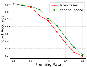
Our channel-based method is compared with the filter-based method [Liu et al., 2017], which evaluate a filter by calculating its absolute weights sum. To validate our method, we prune some filters from a pre-trained VGG-16 on CIFAR-10 without applying the recovery mechanism. Different layers are pruned with the same pruning rate. Then we fine-tune the pruned model for 1 epoch. The experiment is repeated 5 times to eliminate the influence of random disturbance, and we report the averaged accuracy on the test set. Figure 4 shows the pruning results with pruning rate ranging from 0.1 to 0.9 while both methods are set with the same configuration. The results reveal that our channel-based filter selection outperforms the filter-based selection method.
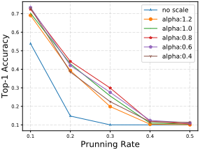
To evaluate the recovery mechanism, we calculate the accuracy of a pruned model on the test set directly without finetuning. Figure 5 indicates that the recovery method helps the pruned model to recover its performance significantly. An impressive result is: while the hyperparameter α in Eq.4 equals to 0.8, the pruned model gets the best recovery. Actually, when we prune a completely unimportant channel, the filter it belongs to does not need to be scaled because the pruned channel almost has no contribution to the whole network performance. Only when it occupies a relatively large proportion of the filter, scaling operation is necessary.
4.3 Results
Our end-to-end layer-selection method is compared to both orderly and global pruning method. Specifically, on the fullyconnected network and VGG, we report the pruning results compared with two global pruning methods [Liu et al., 2017; Wen et al., 2016]. On the Resnet-56, we compare with an orderly pruning method [Li et al., 2017] because the global pruning leads to more performance loss on deeper networks.
VGG-19 on CIFAR-10
We prune the VGG-19 [Simonyan and Zisserman, 2015] on the CIFAR-10 dataset. Each convolution layer is followed by a batch normalization layer [Ioffe and Szegedy, 2015] and we remove its FC layers except the last layer for classification.
Floating-point operations per second(FLOPs) is used as an indicator of model complexity. One multiply-add here is regarded as a floating-point operation unit. We calculate the reward R according to Eq. 1 where network's accuracy in validation set represents performance, FLOPs represents complexity and λ is set to 4 × 10⁻¹⁰ .
| Model | FLOPs | Pruned Rate% | Acc.% |
|---|---|---|---|
| Baseline | 3.9 × 10⁸ | - | 93.66 |
| Slimming-4 | - | 77.2 | -0.25 |
| Slimming-5 | - | 88.7 | -1.39 |
| Ours | 5.98 × 10⁷ | 84.7 | -0.36 |
| Model | FLOPs | Pruned Rate% | Acc.% |
|---|---|---|---|
| Baseline | 3.9 × 10⁸ | - | 73.26 |
| Slimming-3 | - | 67.3 | -2.34 |
| Slimming-4 | - | 83 | -3.85 |
| Ours | 1.19 × 10⁷ | 70.1 | +0.0 |
We summarize the results in Table 1 comparing our method with the global slimming method [Liu et al., 2017], which select unimportant filters in all the layers first and then prune all of them simultaneously. "Slimming-N" denotes repeating the slimming method N times. After LSTM is trained for 150 epochs, the optimal structure emerges, whose FLOPs is reduced by 84.7% with only 0.36% accuracy decrease.
It is worth noting that [Liu et al., 2017] take one multiplyadd as two floating-point operations, so their calculated FLOPs is two times as much as ours. For a fair and clear comparison, our FLOPs calculation method is regarded as a unified standard. Table 1 displays the standardized results.
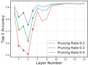
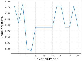
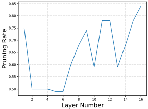
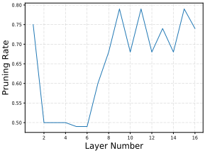
For further investigation, we plot the sensitivity of each layer in the pre-trained VGG-19 in Figure 6. Specifically, at each time we prune one layer while keeping the other layers unchanged, then calculate the accuracy. The results depict that the overall sensitivity distribution keeps the same under different pruning rates and the most sensitive four layers are layer 2,3,4,5. Figure 7, Figure 8 and Figure 9 represent the practical pruning rate of each layer for the optimal network after training LSTM for 50, 150 and 250 epochs respectively. With more training, the real pruning rate from layer 2 to 5 becomes lower and the other layers are pruned more, which is consistent with the observation from Figure 6. The results demonstrate that our method could make reasonable pruning decisions and learn the network sensitivity effectively.
VGG-19 on CIFAR-100
We use the same VGG-19 network to evaluate our method on CIFAR-100. Due to more categories, CIFAR-100 is much more difficult to train than CIFAR-10. Thus, the training and validation set are both used to fine-tune the pruned model. Here we use the training loss to evaluate performance, and set λ to 2 × 10-11 in Eq. 1. After training LSTM for 123 epochs, we get the best network whose FLOPs is reduced by 70.1% with no accuracy drop. As can be seen from Table 2, our method outperforms the slimming method significantly.
ResNet-56 on CIFAR-10
In this section, we verify the feasibility of our method on ResNet-56 [He et al., 2016]. Due to the particularity of ResNet structure, we only prune the first convolution layer of each ResNet block and keep the second convolution layer unchanged for its correctness. The parameter configuration of Eq. 1 is the same as the VGG-19 experiment on CIFAR-10.
| Model | FLOPs | Pruned Rate% | Acc.% |
|---|---|---|---|
| Baseline | 1.25 × 10⁸ | - | 93.04 |
| Li-A | - | 10.4 | +0.06 |
| Li-B | - | 27.6 | +0.02 |
| Ours-2 | 8.24 × 10⁷ | 34.1 | +0.56 |
| Ours-1 | 6.56 × 10⁷ | 47.5 | -0.11 |
| Model | Pruned% | Acc.% | #Neurons |
|---|---|---|---|
| Baseline | - | 98.57 | 784-500-300-10 |
| Structured sparsity | 83.5 | -0.11 | 434-174-78-10 |
| Slimming-1 | 84.4 | -0.06 | 784-100-60-10 |
| Ours | 87.26 | -0.03 | 784-83-48-10 |
Table. 3 reports our results compared to [Li et al., 2017], which analyze the sensitivity of each ResNet block first, then prune filters referring to the analysis results. We do not make any analysis in advance because our method is capable of automatically learning the network sensitivity. After LSTM is trained for 32 epochs, the best network emerges with 47.5% FLOPs reduction and comparable accuracy. Compared to [Li et al., 2017], more filters are pruned with acceptable accuracy decrease of 0.11%. For further comparison, we select the second-best structure with less FLOPs reduction, and it achieves a notable 0.56% accuracy promotion.
Although [Li et al., 2017] set different pruning rates for different layers manually, they prune filters layer by layer. Our method breaks the traditional thinking of pruning a model in the sequential order and works better in practice.
A Fully-connected Network on MNIST
We further validate the effect of our method on multi-layer perceptrons. We prune a 3-layer fully-connected network compared with two global pruning methods [Wen et al., 2016; Liu et al., 2017] as shown in Table 4. Similar to CNNs, the evaluation of neurons in the current FC layer depends on its next FC layer. Here we use the accuracy on the validation set to measure performance. We set λ to 1 × 10⁻⁷ . After 20 epochs, the optimal network structure emerges with 87% neurons pruned and only 0.03% accuracy drop.
5 Conclusion
In this paper, we propose a framework to evaluate the importance of each network layer and to select the most unimportant layers to prune. Considering the hierarchical structure of CNNs, we employ LSTM as an evaluation model to generate the pruning decisions. Besides, the channel-based filter selection method and recovery mechanism are adopted to prune filters effectively. Experimental results show the superiority compared to both orderly and global pruning methods and reveal the ability to learn the sensitivity of each network layer.
@inproceedings{ijcai2018p445,
  title     = {Where to Prune: Using LSTM to Guide End-to-end Pruning},
  author    = {Zhong, Jing and Ding, Guiguang and Guo, Yuchen and Han, Jungong and Wang, Bin},
  booktitle = {Proceedings of the Twenty-Seventh International Joint Conference on
               Artificial Intelligence, {IJCAI-18}},
  publisher = {International Joint Conferences on Artificial Intelligence Organization},
  editor    = {Jérôme Lang},
  pages     = {3205--3211},
  year      = {2018},
  month     = {7},
  note      = {Main track},
  doi       = {10.24963/ijcai.2018/445},
  url       = {https://doi.org/10.24963/ijcai.2018/445},
}
TY - CPAPER TI - Where to Prune: Using LSTM to Guide End-to-end Pruning AU - Zhong, Jing AU - Ding, Guiguang AU - Guo, Yuchen AU - Han, Jungong AU - Wang, Bin T2 - Proceedings of the Twenty-Seventh International Joint Conference on Artificial Intelligence, IJCAI-18 PB - International Joint Conferences on Artificial Intelligence Organization PY - 2018 SP - 3205 EP - 3211 DO - 10.24963/ijcai.2018/445 UR - https://doi.org/10.24963/ijcai.2018/445 ER -Copied
Machine-readable versions of this paper, for tools and AI agents:





