
MUSCAT: Multi-Scale Spatio-Temporal Learning with Application to Climate Modeling
Proceedings of the Twenty-Seventh International Joint Conference on Artificial Intelligence. Main track. Pages 2912-2918.
https://doi.org/10.24963/ijcai.2018/404
Keywords
- Machine Learning: Feature Selection ; Learning Sparse Models
- Machine Learning: Transfer, Adaptation, Multi-task Learning
Abstract
In climate and environmental sciences, vast amount of spatio-temporal data have been generated at varying spatial resolutions from satellite observations and computer models. Integrating such diverse sources of data has proven to be useful for building prediction models as the multi-scale data may capture different aspects of the Earth system. In this paper, we present a novel framework called MUSCAT for predictive modeling of multi-scale, spatio-temporal data. MUSCAT performs a joint decomposition of multiple tensors from different spatial scales, taking into account the relationships between the variables. The latent factors derived from the joint tensor decomposition are used to train the spatial and temporal prediction models at different scales for each location. The outputs from these ensemble of spatial and temporal models will be aggregated to generate future predictions. An incremental learning algorithm is also proposed to handle the massive size of the tensors. Experimental results on real-world data from the United States Historical Climate Network (USHCN) showed that MUSCAT outperformed other competing methods in more than 70\% of the locations.
- [Acar et al., 2011] Evrim Acar, Tamara G. Kolda, and Daniel M. Dunlavy. All-at-once optimization for coupled matrix and tensor factorizations. In MLG'11: Proceedings of Mining and Learning with Graphs, August 2011.
- [Bellocchio et al., 2012] F. Bellocchio, S. Ferrari, V. Piuri, and N.A. Borghese. Hierarchical approach for multiscale support vector regression. IEEE TNNLS, 23(9):1448- 1460, September 2012.
- [Bertasius et al., 2015] Gedas Bertasius, Jianbo Shi, and Lorenzo Torresani. Deepedge: A multi-scale bifurcated deep network for top-down contour detection. In CVPR, pages 4380-4389, 2015.
- [Caruana, 1997] Rich Caruana. Multitask learning. Machine Learning, 28(1):41-75, July 1997.
- [Eigen et al., 2014] David Eigen, Christian Puhrsch, and Rob Fergus. Depth map prediction from a single image using a multi-scale deep network. In NIPS, pages 2366-2374, 2014.
- [Ermiş et al., 2015] Beyza Ermiş, Evrim Acar, and A. Taylan Cemgil. Link prediction in heterogeneous data via general- ized coupled tensor factorization. Data Mining and Knowl- edge Discovery, 29(1):203-236, Jan 2015.
- [Gonçalves et al., 2016] André R. Gonçalves, Fernando J. Von Zuben, and Arindam Banerjee. Multi-task sparse structure learning with gaussian copula models. JMLR, 17(1):1205-1234, January 2016.
- [Gonçalves et al., 2017] André R. Gonçalves, Arindam Banerjee, and Fernando J. Von Zuben. Spatial projection of multiple climate variables using hierarchical multitask learning. In AAAI, pages 4509-4515, 2017.
- [Kolda and Bader, 2009] Tamara G. Kolda and Brett W. Bader. Tensor decompositions and applications. SIAM Re- view, 51(3):455-500, August 2009.
- [Miller et al., 2015] Bradley A. Miller, Sylvia Koszinski, Marc Wehrhan, and Michael Sommer. Impact of multi- scale predictor selection for modeling soil properties. Geo- derma, 239-240:97 -106, 2015.
- [Neverova et al., 2014] Natalia Neverova, Christian Wolf, Graham W. Taylor, and Florian Nebout. Multi-scale deep learning for gesture detection and localization. In ECCV Workshops, pages 474-490, 2014.
- [Nounou and Nounou, 2010] Mohamed N. Nounou and Hazem N. Nounou. Multiscale latent variable regression. International Journal of Chemical Engineering, 2010, 2010.
- [Parikh and Boyd, 2014] Neal Parikh and Stephen Boyd. Proximal algorithms. Foundations and Trends in Opti- mization, 1(3):127-239, January 2014.
- [Steinbach et al., 2003] Michael Steinbach, Pang-Ning Tan, Vipin Kumar, Steven Klooster, and Christopher Potter. Discovery of climate indices using clustering. In KDD, pages 446-455, 2003.
- [Sun et al., 2008] Jimeng Sun, Dacheng Tao, Spiros Pa- padimitriou, Philip S. Yu, and Christos Faloutsos. Incre- mental tensor analysis: Theory and applications. TKDD, 2(3):11:1-11:37, 2008.
- [Walder et al., 2008] Christian Walder, Kwang In Kim, and Bernhard Schölkopf. Sparse multiscale gaussian process regression. In ICML, pages 1112-1119, 2008.
- [Xu et al., 2016a] Jianpeng Xu, Pang-Ning Tan, Lifeng Luo, and Jiayu Zhou. Gspartan: a geospatio-temporal multi-task learning framework for multi-location prediction. In SDM, pages 657-665, 2016.
- [Xu et al., 2016b] Jianpeng Xu, Jiayu Zhou, Pang-Ning Tan, Xi Liu, and Lifeng Luo. Wisdom: Weighted incremental spatio-temporal multi-task learning via tensor decomposi- tion. In IEEE Big Data, pages 522-531, Dec 2016.
- [Xu et al., 2017] Jianpeng Xu, Pang-Ning Tan, Jiayu Zhou, and Lifeng Luo. Online multi-task learning framework for ensemble forecasting. IEEE TKDE, 29(6):1268-1280, 2017.
- [Yu et al., 2015] Rose Yu, Dehua Cheng, and Yan Liu. Ac- celerated online low rank tensor learning for multivariate spatiotemporal streams. In ICML, volume 37, pages 238- 247, 2015.
- [Zhao and Du, 2016] Wenzhi Zhao and Shihong Du. Learn- ing multiscale and deep representations for classifying re- motely sensed imagery. JPRS, 113:155 -165, 2016.
- [Zhao et al., 2015] Liang Zhao, Qian Sun, Jieping Ye, Feng Chen, Chang-Tien Lu, and Naren Ramakrishnan. Multi- task learning for spatio-temporal event forecasting. In KDD, pages 1503-1512, 2015.
- [Zhou et al., 2016] Shuo Zhou, Xuan Vinh Nguyen, James Bailey, Yunzhe Jia, and Ian Davidson. Accelerating Online CP Decompositions for Higher Order Tensors. In KDD, pages 1375-1384, 2016.
References were extracted automatically from the PDF and may contain errors.
Full text extracted automatically from the PDF; figures, tables and equations may differ. The PDF is the version of record.
1 Introduction
The spatio-temporal data obtained from climate and environmental sciences are often available at multiple spatial resolutions. For example, Table ?? shows examples of climate data generated by different global and regional climate models, which can have varying spatial scales, from tens to several hundred kilometers. Such multi-scale data provide useful information that can aid scientists in understanding the variability of the climate system in order to predict its future behavior. However, since the data at different scales are potentially correlated with each other, concatenating them together into a single feature vector may not be an effective strategy for building robust prediction models. Utilizing only the data from the finest resolution is also not a viable approach as the data at coarser resolutions may capture broad-scale effects that cannot be easily discerned from the finest resolution data. Finding an effective way to integrate the multi-scale data into a prediction modeling framework is thus a challenge that needs to be addressed [Miller et al., 2015].
| Climate Dataset | Scale |
|---|---|
| NCEP North American Regional Reanalysis Canadian Regional Climate Model Weather Research & Forecasting Model | 32 km |
| 45 km | |
| 50 km | |
| HadCM3 Global Climate Model | 300 km |
For applications such as climate modeling, in addition to the multi-scale nature of the data, the predictions must be made at multiple locations. Although a model can be trained to fit the training data at each location independently, the output predictions may not be spatially coherent as the models may not preserve the spatial autocorrelation of the data. Furthermore, the amount of training data may vary from one location to another, making it difficult to obtain accurate models for locations with limited training data. Recent works have demonstrated the advantages of applying multi-task learning to such multi-location prediction problems [Xu et al., 2016a][Xu et al., 2016b][Gonçalves et al., 2016][Gonçalves et al., 2017][Yu et al., 2015]. These approaches consider the spatial relationship between different locations to jointly train the models. However, none of them are designed to handle multi-scale data. Furthermore, these approaches are mostly developed for batch learning algorithms, making it harder to scale them up to larger spatio-temporal datasets.
Finally, model interpretability is also important for many spatio-temporal applications. For example, climate scientists are interested to understand the major driving factors that influence the climate variability at various locations. Some of the factors, such as the El Niño phenomenon, are well-known to the scientists, but there may be other broad-scale patterns governing the variability of the data. Thus, it would be useful to develop a framework that can shed light on these patterns in addition to generating accurate predictions.
To address these challenges, this paper presents a novel framework called MUSCAT (MUlti-SCAle Spatio-Temporal Learning) for the predictive modeling of multi-scale spatiotemporal data. MUSCAT represents the spatio-temporal data at each scale as a 3-dimensional tensor. The tensors are then jointly decomposed into a set of shared latent factors, representing the various patterns that can help summarize the variability observed in the spatio-temporal data. MUSCAT employs an ensemble of spatial and temporal prediction models to make its predictions, where the spatial models are trained to fit the climate response variable against the shared spatial latent factors of the tensors whereas the temporal models are trained to fit the respective temporal latent factors. More importantly, the multi-scale tensor decomposition and the fitting of spatial and temporal prediction models are performed simultaneously in a unified learning framework. As this can be computationally expensive due to the massive size of the spatio-temporal data, an incremental learning algorithm is proposed. The algorithm enables the latent factors and model parameters to be iteratively learned over space and time, thereby avoiding the need to rebuild the models from scratch each time there is new data available.
In short, the main contributions of this work are:
- A novel framework called MUSCAT is proposed for the predictive modeling of multi-scale spatio-temporal data. The framework allows the latent spatial and temporal patterns shared by the multiple scales to be simultaneously derived using a multi-tensor decomposition approach. MUSCAT also trains an ensemble of spatial and temporal prediction models, whose outputs will be aggregated when making predictions for a new location or for a future time period.
- To improve its scalability, an incremental learning algorithm over space and time is proposed.
- Experiments performed on real-world data from the United States Historical Climate Network (USHCN) demonstrates the superiority of MUSCAT compared to other competing algorithms.
2 RelatedWorks
This section reviews some of the previous works related to this research. In recent years, multi-task learning has been proven to be effective at learning models for predicting multiple tasks jointly by taking into account the relationships among the tasks [Caruana, 1997]. The success of multi-task learning for spatio-temporal data has also been been demonstrated in [Xu et al., 2017][Xu et al., 2016a][Xu et al., 2016b][Zhao et al., 2015][Yu et al., 2015]. However, none of these approaches are designed for multi-scale data.
The term multi-scale learning has been used rather loosely in the literature to describe different classes of methods. For example, in traditional machine learning, it has referred to techniques based on multiple kernels [Bellocchio et al., 2012], multi-covariance matrices [Walder et al., 2008] or multi-basis functions [Nounou and Nounou, 2010], none of which are designed to handle multi-scale data. Instead, they were developed to extract multi-scale features from the given data. A closer related area is in deep learning, where multiscale modeling approaches have been developed for computer vision applications. Here, the multi-scale data refer to different resolutions of an image [Bertasius et al., 2015; Zhao and Du, 2016]. Other multi-scale learning approaches, such as those proposed in [Neverova et al., 2014] and [Eigen et al., 2014] do not consider the relationships between data at different scales.
Tensor decomposition has been widely used to explore the latent features of multi-dimensional data [Kolda and Bader, 2009]. This includes previous works on coupled tensor decomposition [Acar et al., 2011; Ermiş et al., 2015] for the joint analysis of data from multiple sources. However, such methods are mostly designed for batch learning, and thus, cannot efficiently handle the dynamic growth of data in different dimensions (e.g., spatial and temporal). As an alternative, incremental or online tensor decomposition approaches have been developed in recent years [Sun et al., 2008; Zhou et al., 2016]. These methods are unsupervised, and thus, are not as effective compared to the MUSCAT framework proposed in this paper. More recently, Yu, et al. [Yu et al., 2015] also presented an online supervised tensor decomposition method. Unlike MUSCAT, the method employed a tensor to represent the model parameters instead of the data. As will be shown in our experiments, the strategy used by MUSCAT to represent data as tensors instead of model parameters as tensors is more effective for modeling the multi-scale spatio-temporal data investigated in this study.
3 ProposedMUSCAT Framework
MUSCAT is a supervised learning framework that jointly performs a coupled tensor decomposition on a multi-scale spatiotemporal dataset and fits the derived latent factors to the response variable of interest at multiple locations. This section presents the details of our proposed framework.
3.1 Preliminaries
Let D = (X (1) , ...,X (L) ,Y) be a multi-scale spatiotemporal data set, where X (l) ∈ ℜS×T×dl denote the spatiotemporal tensor of predictor variables at the l-th scale, Y ∈ ℜS×T denote the time series of the response variable for all locations, S is the number of locations, T is the length of time series, and dl is the number of predictor variables associated with the l-th scale.
Inspired by previous work on discovering climate indices using SVD [Steinbach et al., 2003], we employ tensor decomposition to extract broad-scale patterns from the spatio-temporal data. Specifically, the following CANDECOMP/PARAFAC (CP) decomposition [Kolda and Bader, 2009] is used to decompose a 3rd-order tensor X into its corresponding latent factors, A, B, and C:
where ak, bk and ck are column vectors corresponding to the k-th columns of matrices A, B, and C, and ◦ denotes the outer product operation.
3.2 Supervised Tensor Decomposition for Multi-Scale Data
For multi-scale spatio-temporal data, the tensor decomposition can be performed at each scale l as follows:
where A ∈ ℜS×K denote the spatial latent factors and B ∈ ℜT×K denote the temporal latent factors. Our framework assumes that the spatial and temporal latent factors A and B are invariant across all scales. The normalization factor vol(l) = 2(S×T ×dl) ensures that the decomposition at each scale does not depend on its tensor size. Finally, Ωd(A, B, C) is the regularization term used to enforce the sparsity of the latent factors:
Although the latent factors derived via multi-tensor decomposition may capture the spatial and temporal variabilities of the data, they may not be well-suited for predictive modeling applications. To overcome this problem, MUSCAT incorporates the multi-tensor decomposition process directly into a supervised learning framework. Specifically, it assumes that the prediction for location s at time t is given by the weighted average of the predictions generated from models trained on data at different scales, i.e., ˆ ys,t = ∑Ll αlˆ y(l) s,t , where αl is the weight associated with the prediction function of the l-th scale. The weights are assumed to form a probability simplex that satisfies αl ≥ 0 and ∑Ll αl = 1.
Furthermore, the prediction model at a given scale l is given by an ensemble of spatial and temporal models:
where x(l) s,t denotes the feature vector for location s and time t at scale l, w(l) k and v(l) k are parameters of the spatial and temporal prediction models for the k-th latent factor, while As,k and Bt,k are the scalar coefficients for the k-th spatial and temporal latent factors associated with location s and time t, respectively. Note that we enforce the constraint that the spatial and temporal latent factors are invariant across all scales, i.e., ∀l : A(l) = A, B(l) = B.
Our framework to simultaneously uncover the latent factors and derive the parameters for the spatial and temporal prediction models can be formalized as follows:
where W, V and C denote the set of W(l) , V(l) and C(l) for l = 1, ..., L respectively for notation simplicity, and ˆY(l) corresponds to the predictions generated by the spatio-temporal models at scale l, as shown in Equation (2). We also use ∥[{W(l) ,V(l) ,C(l) },A, B]∥1 to denote the ℓ1 norm regularization term for W(l) , V(l) , A, B and C(l) , respectively.
3.3 Incremental Learning
Optimizing Eq. (3) can be expensive for large spatiotemporal data. The problem is further exacerbated by the fact that the data may grow over time. Learning the model from scratch whenever there are new data available is not a feasible solution. In this section, we present an efficient algorithm to learn the model parameters and latent factors incrementally over space or time without requiring the memory of old data. Let Dnew = (X new,Y new) denote the set of new observations and ˜Π = {˜α, ˜W, ˜V, ˜C, ˜A, ˜ B} be the previous set of model parameters and latent factors estimated by the algorithm. For incremental learning, the model parameters and latent factors are updated by optimizing the following objec-
tive function:
where F(Π; Dnew) is given by Eq.(3) and
is a regularization term to ensure smoothness of the model by controlling the amount of information to be retained from the previous model. Our formulation enables the update formula to be applied when augmented with data from new locations or when data for a new time period become available. We consider the former as incremental learning over space and the latter as incremental learning over time.
Incremental Learning over Space
Let T be the current time step and S be the number of locations with training data at time T . Without loss of generality, we assume that the model is updated with new data one location at a time. Furthermore, the historical data for the new location is assumed to be available from time t0 to T. If the location has only one historical observation, then t0 = T. For brevity, we denote the multi-scale tensor data for the new location as X (l) S+1 ∈ ℜ1×(T-t0+1)×dl for l = 1, ...,L, and d = ∑Ll=1 dl. With the addition of the new data, the spatial latent factors need to be updated from its previous matrix ˜AS ∈ ℜS×K to AS+1 ∈ ℜ(S+1)×K = [AS; aTS+1 ]. We further assume that the spatial latent factors for other locations are unaffected by the addition of the new location, i.e., AS = ˜AS. However, the latent factors for other modes of the tensor (B and C(l) ) as well as the parameters of the prediction models (αl, W(l) and V(l) ) can be affected by the addition of the new data.
for incremental learning over space is:
where aS+1 is a column vector that represents the spatial latent factors for the new location. The smoothness parameter η1 determines the extent to which the previous model parameters should be retained.
An alternating minimization strategy is used to solve the optimization problem, and each subproblem is solved by the proximal gradient descent method [Parikh and Boyd, 2014]. The parameters are updated iteratively by calculating the gradient on the smooth part of the objective function, and then apply the soft-thresholding operator to determine its next value. The step size can be found using a line search algorithm. The details of the gradient calculation is omitted in this paper due to the space limitation.
Incremental Learning over Time
MUSCAT performs incremental learning over time when there are new observations available at the new timestamp. Let S be the number of locations and T be the current time. We denote the newly acquired data for all S stations at time T + 1 as {X (1) T +1 , X (2) T+1 , · · · ,X (L) T+1 }, where each X (l) T+1 ∈ ℜS×1×dl corresponds to the data at scale l and d = ∑Ll=1 dl. We use this information to update the temporal latent factors from ˜BT ∈ ℜT×K to BT+1 ∈ ℜ(T+1)×K = [BT ; bTT+1 ]. Similar to the strategy for incremental learning over space, we assume the new data for time T + 1 does not affect previous temporal latent factors: BT = ˜BT .
Incremental learning over time is implemented via the following two steps. First, we learn the temporal latent factor bT+1 based on the predictor variables for the new time period before the target variable is observed. Next, the parameters and latent factors for other modes are updated when the target variable for the new time period is observed for all the locations.
Step 1: Updating the temporal latent factor bT+1. The objective function for updating bT+1 is:
Note that A and {C(l) } correspond to the matrices obtained from the previous update. The predictions for the target variable are performed using bT+1 and other model parameters from previous update.
Step 2: Updating model parameters and latent factors after observing target variable. After observing the true values of the target variable at time T +1, the model parameters and other latent factors are updated by minimizing the following objective function:
4 Experimental Evaluation
This section describes the extensive experiments performed to demonstrate the effectiveness of MUSCAT when applied to a multi-scale climate dataset.
4.1 Climate Data
The climate data used in our experiments has three spatial resolutions. At the finest scale, monthly climate data are obtained for more than 300 weather stations from the United States Historical Climatology Network (USHCN) 1 . Four variables-maximum (tmax), minimum (tmin), mean (tmean) temperature and precipitation (prcp)-are selected as response variables for our prediction task. We train a prediction model for each response variable separately.
We use two gridded climate datasets, NARR and NCEP reanalysis, to create the predictor variables. NARR 2 , which stands for the North American regional reanalysis dataset, has a spatial resolution of 0.3◦ (32 km) whereas NCEP reanalysis 3 has a coarser resolution of 2.5◦ . Nine variables fromNARR (acpcp, air.2m, dlwrf, dswrf, lftx4, prate, prmsl, pr_wtr, and rhum) along with seven variables from NCEP reanalysis (cprat.sfc, dlwrf.sfc, dswrf.sfc, prate.sfc, tmax.2m, tmin.2m, and lftx.sfc) are chosen as predictor variables.
The monthly climate data span a 30-year period between January 1985 to November 2015. Table 2 shows the number of stations and grid cells, which may vary for each response variable since we discard stations with missing values. The time series for the predictor and response variables are deseasonalized (by subtracting each monthly value from the mean of its corresponding month) and subsequently standardized.
1 http://cdiac.ornl.gov/epubs/ndp/ushcn/ushcn.html
2 https://www.esrl.noaa.gov/psd/data/gridded/data.narr.html
3 http://www.esrl.noaa.gov/psd/data/gridded/data.ncep. reanalysis.derived.html
| USHCN | NARR | NCEP | |
|---|---|---|---|
| tmax | 357 | 350 | 146 |
| tmin | 341 | 336 | 144 |
| tmean | 333 | 328 | 143 |
| prcp | 790 | 635 | 159 |
4.2 Experimental Setup
The 30-year climate dataset is divided into 3 partitions. We first incrementally build the models using training data from the first 10 years (1985-1994) and then apply the models to validation data from the next 10 years (1995-2004). After tuning the model hyperparameters using the validation set, we apply the chosen models to data from the last 10 years (20052015), which serve as our test set. Note that the number of weather stations associated with the training, validation, and test sets may vary depending on when each station was introduced into the incremental learning process. Initially, we randomly choose 100 weather stations as our starting locations. At each step of the incremental learning process, we randomly add either a new station or a new time period to update the latent factors and the ensemble of prediction models.
We used the mean absolute error (MAE) metric to evaluate the performance of various algorithms:
Note that the MAE is calculated for each station s starting from its corresponding test period ts. For example, if a station was introduced into the incremental learning formulation during the training or validation period, then its MAE is calculated for the entire 10-year test period. However, if the station was first introduced during the testing period, its MAE is computed starting from the time it was introduced. The incremental learning process is repeated 10 times, each time with a different initialization and random ordering of weather stations. Results are reported based on the average performance over the 10 trials.
4.3 Baseline Algorithm
We compare the performance of MUSCAT against the following three incremental learning algorithms.
- STL (Single Task Learning): A linear model is incrementally trained at each location using the stochastic gradient descent algorithm. When a new weather station is introduced during the incremental learning process, its model parameters are initialized randomly and updated as new observation data become available.
- ALTO: This is variation of the spatio-temporal multitask learning algorithm proposed in [Yu et al., 2015] which was designed to build models for multiple response variables simultaneously.
- WISDOM: This is a recent spatio-temporal multi-task learning approach [Xu et al., 2016b] that applies tensor decomposition on the data but does not distinguish between variables from different scales.
4.4 Experimental Results
We designed our experiments to (1) compare the performance of MUSCAT against the baseline methods, (2) assess the value of using multi-scale data, and (3) analyze the significance of the latent factors.
Comparison against Baseline Methods
Table 3 shows the mean and standard deviation of MAE after 10 trials for each method. The results suggest that WISDOM and MUSCAT significantly outperform STL and ALTO in all four datasets, which suggests the advantages of using a multitask learning approach based on tensor decomposition. In addition, MUSCAT outperforms WISDOM on all four datasets in this study, which shows the benefits of using our approach to factorize the multi-scale tensors jointly, instead of factorizing a single tensor with concatenated features from all scales, which is the approach used in WISDOM. A more detailed analysis given in Table 5 shows that MUSCAT outperforms all other competing methods in at least 70% of the stations for all 4 response variables.
Value of Multi-scale Data
To determine the value of using multi-scale data, we consider the following two variations of MUSCAT: (1) MUSCATS1, which uses only predictor variables from NCEP, and (2) MUSCAT-S2, which uses only predictor variables from NARR. Once again, the results shown in Table 4 suggest that MUSCAT outperforms WISDOM, MUSCAT-S1, and MUSCAT-S2 on all four datasets. For temperature predictions, WISDOM is superior than MUSCAT-S1 and MUSCATS2, which shows the importance of incorporating data from all scales into the learning framework. However, for precipitation prediction, MUSCAT-S2 outperforms WISDOM, which indicates that augmenting the predictor variables from the coarsest scale may degrade the model performance. Nonetheless, MUSCAT still achieves the lowest MAE because it can learn the appropriate weight (α) for combining the predictions from NARR and NCEP reanalysis datasets. To measure the relative influence of data at different scales on the performance of MUSCAT, we examine the mean values of the parameters α1 and α2 over the 10 trials. The results given in Table 6 suggest that α2, which is the weight associated with the finer-level predictors, has a consistently higher weight than α1, the weight associated with coarser-level predictors on all four datasets. This shows that the finer-level predictors have higher impact on the prediction than coarser-level predictors.
4.5 Analysis of Latent Factors
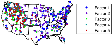
One of the advantages of using MUSCAT is that the latent factors can be used to identify the spatial patterns of the data. To illustrate this, Figure 1 shows the spatial distribution of the latent factors for precipitation data. For each spatial latent factor, we plot its top 20% most influential stations on the map. The results suggest that the latent factors exhibit some spatially coherent patterns. For example, the first latent factor is more dominant on the eastern part of the United States, while the third and fifth latent factors are more influential on the northwest part of the country.
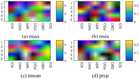
We also examine the temporal latent factors derived by MUSCAT by computing their pairwise absolute correlation against some of the well-known climate indices, such as AOI, NAO, WPI, QBO, PDO, and SOI (details of these climate indices are shown in Table 7). The results are shown in Figure 2. The correlation values are not that high, which is not surprising as the study region is limited to the United States only.
| tmax | tmin | tmean | prcp | |
|---|---|---|---|---|
| STL | 0.4422 ± 0.0016 | 0.4412 ± 0.0020 | 0.4141 ± 0.0018 | 0.5446 ± 0.0012 |
| ALTO | 0.5854 ± 0.0064 | 0.5687 ± 0.0031 | 0.5656 ± 0.0053 | 0.5806 ± 0.0051 |
| WISDOM | 0.3543 ± 0.0155 | 0.4001 ± 0.0075 | 0.3850 ± 0.0236 | 0.4212 ± 0.0054 |
| MUSCAT | 0.3212 ± 0.0074 | 0.3454 ± 0.0065 | 0.2844 ± 0.0112 | 0.4115 ± 0.0023 |
| tmax | tmin | tmean | prcp | |
|---|---|---|---|---|
| WISDOM | 0.3543 ± 0.0155 | 0.4001 ± 0.0075 | 0.3850 ± 0.0236 | 0.4212 ± 0.0054 |
| MUSCAT-S1 | 0.5492 ± 0.0700 | 0.4328 ± 0.0115 | 0.4543 ± 0.0393 | 0.6194 ± 0.0026 |
| MUSCAT-S2 | 0.3910 ± 0.0183 | 0.4094 ± 0.0186 | 0.4350 ± 0.0532 | 0.4208 ± 0.0051 |
| MUSCAT | 0.3212 ± 0.0074 | 0.3454 ± 0.0065 | 0.2844 ± 0.0112 | 0.4115 ± 0.0023 |
| total # stations | STL | ALTO | WISDOM | |
|---|---|---|---|---|
| tmax | 357 | 355 | 315 | 350 |
| tmin | 341 | 330 | 321 | 339 |
| tmean | 333 | 331 | 313 | 333 |
| prcp | 790 | 780 | 739 | 553 |
| tmax | tmin | tmean | prcp | |
|---|---|---|---|---|
| α1 | 0.2876 | 0.3651 | 0.3360 | 0.0933 |
| α2 | 0.7124 | 0.6349 | 0.6640 | 0.9067 |
5 Conclusion
This paper presents a multi-scale multi-task learning framework for geospatio-temporal data by employing a supervised multi-tensor decomposition approach. The framework enables the multi-scale relationships to be harnessed by enforcing a constraint on the consistency between the spatial and temporal latent factors derived from the multi-scale geospatio-temporal data. An incremental learning algorithm over space and time is then proposed to efficiently learn the weights of the model. Experiments performed on a real-world multi-scale climate dataset demonstrate the effectiveness of proposed method compared to several baseline algorithms.
| Climate Index | Description |
|---|---|
| AOI | Arctic Oscillation Index |
| NAO | North Atlantic Oscillation |
| WPI | West Pacific Pattern |
| QBO | Quasi-Biennial Oscillation |
| PDO | Pacific Decadal Oscillation |
| SOI | Southern Oscillation Index |
@inproceedings{ijcai2018p404,
  title     = {MUSCAT: Multi-Scale Spatio-Temporal Learning with Application to Climate Modeling},
  author    = {Xu, Jianpeng and Liu, Xi and Wilson, Tyler and Tan, Pang-Ning and Hatami, Pouyan and Luo, Lifeng},
  booktitle = {Proceedings of the Twenty-Seventh International Joint Conference on
               Artificial Intelligence, {IJCAI-18}},
  publisher = {International Joint Conferences on Artificial Intelligence Organization},
  editor    = {Jérôme Lang},
  pages     = {2912--2918},
  year      = {2018},
  month     = {7},
  note      = {Main track},
  doi       = {10.24963/ijcai.2018/404},
  url       = {https://doi.org/10.24963/ijcai.2018/404},
}
TY - CPAPER TI - MUSCAT: Multi-Scale Spatio-Temporal Learning with Application to Climate Modeling AU - Xu, Jianpeng AU - Liu, Xi AU - Wilson, Tyler AU - Tan, Pang-Ning AU - Hatami, Pouyan AU - Luo, Lifeng T2 - Proceedings of the Twenty-Seventh International Joint Conference on Artificial Intelligence, IJCAI-18 PB - International Joint Conferences on Artificial Intelligence Organization PY - 2018 SP - 2912 EP - 2918 DO - 10.24963/ijcai.2018/404 UR - https://doi.org/10.24963/ijcai.2018/404 ER -Copied
Machine-readable versions of this paper, for tools and AI agents:





