Online Continuous-Time Tensor Factorization Based on Pairwise Interactive Point Processes

1 Introduction

Exploring latent structure in real-world multimodal data (i.e., tensors) is a significant problem for analysis of underlying generative mechanisms and for predicting unobserved instances. Tensor factorization (TF) provides a flexible and effective way to learn such latent structure, decomposing the data into latent factors. Tensor factorization has been widely used in many applications and has achieved encouraging performance, e.g., for recommendation systems [Rendle and Schmidt-Thieme, 2010], signal processing [Ozerov et al., 2011], and computer vision [Shashua and Hazan, 2005].

Such data are often observed sequentially, and may be analyzed as multimodal event sequences in continuous time. For example, user behavior in a social network can be treated as a multimodal event (i.e., message sender × message receiver × message type) with a time stamp, and the collection of such events can be formulated as a tensor whose elements contain the counts of the events up to a certain time. This tensor is time-varying, and the relationships between its modalities can change. Accordingly, its latent factors are likely to evolve over time. Therefore, we seek the development of i) a continuous-time tensor factorization (CTTF) for multimodal event sequences; and ii) a method for updating the model online, capturing the evolution of the latent factors over time.

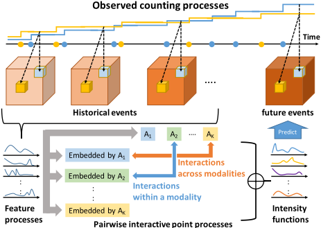
To address these desiderata, we present an online continuous-time tensor factorization method, based on a novel model called pairwise interactive point process. As shown in Fig. 1, the target continuous-time tensor is represented as a set of counting processes, corresponding to multimodal events. The intensity functions of these counting processes are factorized in a pairwise manner, simultaneously representing interactions within each factorization modality and across different modalities, by the inner products of latent factors. Each latent factor is a function of time and embedded features, capturing influences of historical events on current and future ones. Based on the model, we can predict the expected number (i.e., counting processes) of future events.

The model is learned by fitting the expected counting process with the observed one, formulated here as a convex optimization problem, solved effectively by online alternating direction method of multipliers (ADMM). We analyze the convergence and the computational complexity of our method, and compare it with the state-of-the-art methods on two realworld datasets. Experiments show that the proposed method achieves superior performance on predicting future events.

2 RelatedWork

2.1 Tensor Factorization

The Tucker decomposition [Tucker, 1966] factorizes a tensor into a smaller core tensor and a latent factor matrix for each modality; this approach may suffer from high computational complexity. To reduce complexity, the canonical decomposition [Kolda and Bader, 2009] assumes the core tensor is diagonal. A pairwise decomposition method is proposed in [Rendle and Schmidt-Thieme, 2010], which further reduces the computational complexity of tensor factorization, and achieves encouraging results in recommendation systems. The tensor factorization methods in [Rai et al., 2015] leverage side information, to improve the learning results. Bayesian tensor factorization methods [Acharya et al., 2015; Charlin et al., 2015] are also used widely, with scalability improved in [Hu et al., 2015] for count data. However, analysis of the continuous-time evolution of tensor factorization, while an important practical problem, is still relatively under-studied. Existing temporal tensor factorization methods mainly combine tensor factorization with time seriesbased models [Xiong et al., 2010; Dunlavy et al., 2011; Rafailidis and Nanopoulos, 2014; Acharya et al., 2015; Charlin et al., 2015], which only address data with discrete time steps or predefined decays [Koren, 2010], rather than continuous-time event sequences. Additionally, few of them consider online learning for tensor factorization.

2.2 Point Processes

Point processes have been considered in many fields, e.g., for analyzing financial [Bacry et al., 2015] and social network [Blundell et al., 2012] data, and in healthcare [Xu and Zha, 2017; Xu et al., 2017a] and recommendation [Wang et al., 2016] systems. To describe the influences of historical events on current and future ones, a series of complicated models (e.g., the Hawkes process [Hawkes, 1971] and the correcting process [Xu et al., 2015; 2017b]) have been proposed. These early works aimed to capture the dynamics of event sequences associated with a single data modality. Based on these models, many extensions have been proposed, to analyze multimodal (tensor) event sequences, e.g., the multitask multi-dimensional Hawkes process [Luo et al., 2015]. Recently, point processes parameterized by embedded features have been proposed [Wang et al., 2016], which model the events associated with features. However, extension of these methods to continuous-time tensor factorization is still an open problem.

Additionally, although methods have been proposed in [Hall and Willett, 2016; Yang et al., 2017] to explore online learning of point processes, these methods only deal with Hawkes processes in a nonparametric manner. The online learning of parametric point processes, with more general formulations, has not been investigated deeply.

3 ProposedModel

3.1 Notations and Problem Statement

Many real-world data are generated sequentially, and can be formulated as a continuous-time event sequence with multiple data modalities (i.e., data may be mapped to a tensor). A

typical example is online shopping records, in which pairs of users and items are listed along with a time stamp. Such data contain two "modalities," corresponding to users and items, and features may be available to describe each transaction.

We describe event sequences with K modalities as a set of triads, denoted {(tn, ζn, fn)}Nn=1 . The time stamp for event n is denoted tn ∈ [0, T ]; ζn = [c1n , ..., cKn ] ∈ C1 × ... × CK represents the multimodal event type, where Ck is the categorical set of the k-th modality and ckn is the index of the event corresponding to the k-th modality; and fn ∈ RD is an event-dependent feature vector.

We represent the event sequence as a continuous-time tensor, i.e., N(t) = [Nζ(t)] ∈ Z|C1|×...×|CK| + , where ζ = [c1 , ..., cK ] represents a particular multimodal event type, |Ck| represents the cardinality of Ck, and Z+ represents nonnegative integers. Each element Nζ(t) is a counting process, recording the number of type-ζ events that have occurred up to time t. For each ζ, the counting process Nζ(t) can be characterized by the expected instantaneous occurrence rate of the event, conditioned on history, called the intensity function:

where Ht = {(tn, ζn, fn)|tn < t} contains historical events before time t. The intensity functions of all types of events formulate a continuous-time intensity tensor Λ(t) = [λζ(t)] ∈ R|C1|×...×|CK| + . In this setup we do not explicitly model feature vectors fn, which are assumed as observed covariates associated with events; however, the intensity function is dependent on prior feature vectors and other characteristics of previous events.

Problem statement: Given observed counting processes N(t), we aim to explore the latent structures of its intensity tensor Λ(t), capture the evolution of the latent structures over time, and predict the number of events in the future.

3.2 Pairwise Interactive Point Processes

The simplest approach for modeling the intensity tensor Λ(t) is to learn each λζ(t) independently [Du et al., 2015]. Such a strategy may be questionable because the modalities of real-world data often have interactions, and hence there is likely statistical dependencies between the set of {λζ(t)}. To overcome this problem, many existing factorization methods, especially those applied in recommendation systems, consider the pairwise interactions between different modalities in an inner product manner. In particular, for a tensor Λ, those methods represent its element λζ as the sum of the inner products of different latent factors, i.e., λζ = ∑k̸=k′ u⊤k,ckuk′ ,ck′ . For the well-known collaborative filtering problem for a 2D matrix (K = 2) [Koren et al., 2009; Park and Chu, 2009], ζ = [c1 , c2 ], with c1 ∈ C 1 and c2 ∈ C 2 . For any λ[c1 ,c2 ] associated with the |C1| × |C2| matrix, the construction λζ = ∑k̸=k′ u⊤k,ckuk′ ,ck′ yields λ[c1 ,c2 ] = u⊤1,c1u2,c2, where the set of vectors {u1,c1}c1∈C1 represent the entities along axis one, and {u2,c2}c2∈C2 represent the entities along axis two. For 3D tensors this approach generalizes to pairwise factorization [Rendle and SchmidtThieme, 2010].

In the above model, λζ(t) only depends on the crossmodality inner products between the elements of ζ. A natural extension is to also include intra-modality terms, as

Interactions across different modalities

where the L-dimensional vector uk,ck(t) with ck ∈ Ck is the time-dependent latent factor corresponding to the index ck of the k-th modality. For k = 1, ...,K, U k (t) = [uk,1(t), ..., uk,|Ck|(t)] ∈ RL×|Ck| is the latent factor matrix corresponding to the k-th modality.

The work in [Wang et al., 2016] also considered a base intensity ηζ(t), like in (2), but in that prior work the base intensity was time-independent. Similar to the work in [Koren, 2010], we represent the base intensity as the sum of the basis corresponding to different modalities (the ηck(t) in (3)). Moreover, to avoid additional parameters, we reuse the latent factors to parameterize the basis (ηck (t) = u⊤k,ck (t)uk,ck (t)). Such a strategy implies that the base intensity reflects the selfinteractions within each modality.

In summary, (2) means that event type ζ = [c1 , ..., cK ] has an expected occurrence rate at time t controlled simultaneously by the interactions within each modality and the interactions across different modalities. Combining (2) with (3), we rewrite (2) as

Like the work in [Du et al., 2015; Xu et al., 2015; Wang et al., 2016], we represent each latent factor uk,ck(t) as a timedependent embedding of observed features:

where Ak ∈ RL×(D+1) is the k-th embedding matrix, the ˆ fck (t) is the weighted sum of the historical feature vectors up to time t, and κ(t) ≥ 0 is a predefined kernel function deciding the weights. We can find that the latent factor uk,ck is the sum of two components: i) a time-invariant component corresponding to the first column of Ak, and ii) a time-varying component corresponding to the multiplication between the remaining D columns of Ak, denoted as A2:D+1 k and the accumulated features, i.e. A2:D+1 k (∑ckn=ck ,tn<t fnκ(t - tn)). To ensure that the intensity function is physically-meaningful, here we require that the elements of all embedding matrices Ak's and features fn's are nonnegative, such that the intensity function is nonnegative as well.

4 Online Continuous-Time Tensor Factorization

4.1 Reformulation of The Problem

Given observed counting process N(t), we aim to learn the intensity tensor Λ(t) and the parameters {Ak}Kk=1 in the model defined by (4)-(5). Unlike maximum likelihood estimation (MLE) proposed in most existing works [Lewis and Mohler, 2011; Luo et al., 2015; Wang et al., 2016], we learn our pairwise interactive point process model as a regularized linear predictor, for efficient online learning. Specifically, instead of maximizing the likelihood of the observed event sequence, we aim to fit the observed counting process N(t) with their expectation E[N(t)], which is estimated by the integration of the intensity tensor, i.e., ∫ T 0 Λ(s)ds. Given the event sequence {(tn, ζn, fn)}Nn=1 , we present the following squared loss function as the objective function:

We use the factor 1 tn to rescale the weight of the n-th estimation error, because the variance of the averaged intensity, i.e., E[ N(t)-E[N(t)] t ]2 is generally bounded.

Minimizing (6) directly is non-convex because it involves the terms like A⊤k Ak′ , k ̸= k′ . Fortunately, we can reformulate the problem as a convex optimization problem by rewriting the intensity function as

Here, Xkk′ = A⊤k Ak′ , Fck ck′ (t) = ˆ fck(t) ˆ f ⊤ ck(t) is the outer product of the accumulated feature and its transpose, and tr(·) calculates the trace of matrix. The parameter, denoted as x ∈ RD′ , D′ = K(K+1)(D+1)2 2 , is a vectorization of all matrices Xkk′ 's, i.e., x = vec({Xkk′}k≥k′). Similarly, ˜ fζ(t) = vec({Fck ck′ }k≥k′) is the vectorized representation of the Fck ck′ (t)'s.

Based on (7), we rewrite the loss function in (6) as

where the vector N tN 0 = [ 1 tn Nζn (tn)] ∈ RN , and the matrix F tN 0 = [ 1 tn ∫ tn 0 ˜ f ⊤ ζn (s)ds] ∈ RN×D′ . Moreover, the parameter vector x has structure. In particular, we can construct a symmetric rank-L matrix X from the parameter vector x as

where x vectorizes the lower triangular submatrices of X. For convenience, we denote the operator that constructs X from x as X = map(x). Considering the nonnegative and low-rank properties of X, the final optimization problem is

where ‖ · ‖∗ calculates the nuclear norm of the matrix. This regularizer imposes a low-rank constraint on X and its significance is controlled by α. By solving (10), we learn the parameters of our point process model as a regularized linear predictor.

4.2 Online Learning Strategy

To track the evolution of the model with new data, we solve the optimization problem in (10) in the framework of online learning. In particular, we can develop an online learning algorithm based on the stochastic alternating direction method of multipliers (ADMM) [Ouyang et al., 2013; Zhong and Kwok, 2014]. In the initial phase, we first estimate the parameters from the observations till time T, denoted as xT . When new events occur in [T, Tnew], we can calculate the new counting processes and the new embedded features quickly, denoted as N Tnew T and F Tnew T . We can then update the parameters by solving

where y is an auxiliary variable and z is a dual variable. The first term corresponds to the squared loss function for the new data, and the subsequent three terms are argumented Lagrangian terms of ordinary ADMM. Additionally, we add ‖x - xT‖22 to ensure that the new estimation should not be too far from the previous one. The weight of this term is controlled by a parameter β. We can minimize (11) by alternating optimization. In the i-th step, we obtain xi by updating xi-1 based on new observations, and the optimization problem is

This problem can be solved efficiently by projected gradient descent. Given xi, we update yi by solving a low-rank approximation problem, and soft-thresholding is applied.

where the operator Sδ(·) shrinks the singular values of the matrix with a threshold δ, and the operators map(·) and vec(·) are defined as previously. Finally, we obtain the new dual variable zi by zi = zi-1 + (xi - yi). The scheme of our algorithm is shown in Algorithm 1, where the operator (·)+ keeps all nonnegative values from changing and sets all negative values to zeros.

It should be noted that for each time Ti we can construct the low-rank symmetric matrix Xi from the estimated parameters, i.e., Xi = map(xi). When the embedding matrices {Ak}Kk=1 in the interval [Ti-1, Ti] are required, according to (9) we can apply the symmetric nonnegative matrix factorization [Kuang et al., 2012] to Xi and obtain them accordingly.

4.3 Prediction of Future Events

After learning the pairwise interactive point process model, we can predict future events. In particular, given the model trained till time T , we can simulate a set of events happening in the following time interval [T + dT] by Ogata's thinning method [Ogata, 1981]. The expected number of the events with a specific type in this target interval is estimated by averaging the increments of the counting processes in different simulation trials.

Algorithm 1 Online CFFT

Input: An initial sequence in [0, T0], parameters α, β, ρ, τ . Output: A set of xi's for different time intervals.

• 1: Initialize x0 = (((F T0 0 )⊤F T0 0 )-1 (F T0 0 )⊤N T0 0 )+,
• 2: y0 = x0, z0 = 0.
• 3: for i = 1, 2, 3, ... do
• 4: Calculate N Ti Ti-1 and F Ti Ti-1 . Set xi = xi-1.
• 5: Φ= (F Ti Ti-1 )⊤F Ti Ti-1 + (ρ + β)I.
• 6: b = (F Ti Ti-1 )⊤N Ti Ti-1 + ρ(yi-1 - zi-1) + βxi-1.
• 7: Projected gradient descent (Inner iterations):
• 8: while not converge do
• 9: Update x by xi = (xi - 2τ (Φxi - b))+.
• 10: Update y by (13).
• 11: Update z by zi = zi-1 + (xi -yi).

5 Further Analysis

5.1 Convexity and Convergence

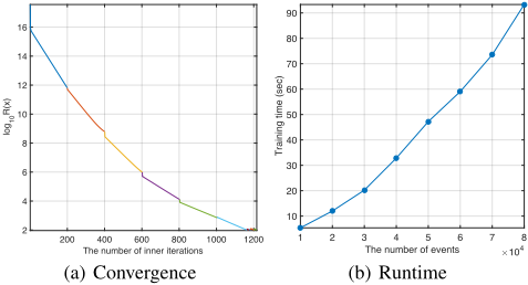
Instead of learning the matrices {Ak}Kk=1 directly, our method reformulates the parameters as a vector x and learns by convex optimization. In the case that the observed event sequences are generated by a stationary point process, the parameters converge to a global optimal solution of (10) with the increase of data. Via the analysis in [Ouyang et al., 2013], the convergence rate of x is guaranteed to be O( log t t ), where t is the number of iterations. Furthermore, even if the target point process is not temporal stationary, our online learning method can still ensure that we can obtain a global optimal solution in each step (i.e., for the data in specific time intervals). In such a situation, the sequence of optimums {xi} reflects the evolution of the target point process. The performance of our method on convergence is shown in Fig. 2(a) for further verification.

5.2 Sample Complexity

Equation (8) measures the empirical risk between the normalized counting processes and their expectations estimated by a linear predictor. According to Theorem 1 in [Shamir, 2015], we have the following proposition:

Proposition 5.1. Suppose N events are observed for a point process with K event types, i.e., ζ ∈ C1 × ... × CK. If its counting process satisfies 1t Nζ(t) < Y for all t and ζ, and its intensity function can be decomposed as in (4), which contains K latent processes with D + 1 dimensions, then we can construct a linear predictor with a D′ -dimensional parameter vector x, where D′ = K(K+1)(D+1)2 2 and ‖x‖2 ≤ B, and the bound on the excess risk E[R(ˆx) -R(x∗ )] satisfies

where ˆx is the optimum learned from observed events and x∗ is the ground truth of the model.

According to (14) we can find that i) when data is insufficient (i.e., N < min{D′ , B2 Y 2 }), the learning results suffers from over-fitting and the excess risk and 1 t2 N 2 ζ (t) have the same order of magnitude; ii) when considering many modalities (i.e., large K) or high-dimensional features (i.e., large D), the bound of excess risk is likely to be O( BY √N ) even if we have a large amount of samples. Fortunately, in many practical applications the number of modalities is limited (K = 2 or 3 commonly) and the low-rank assumption of latent processes is applied, so that the bound O( B2+D′ Y 2 log(1+ N D′ ) N ) is achievable when sufficient events are observed.

5.3 Computational Complexity

The bottleneck of our method is calculating the matrix F Ti Ti-1 in each step. Each row of F Ti Ti-1 involves the integration of intensity function, which considers all events happening before a specific time t. The computation becomes intractable with the increase of historical events. This problem can be solved when defining the kernel function κ(t) in (5) as a monotonically-decreasing function, e.g., exponential function. In particular, we set κ(t) = wexp(-wt), t ≥ 0. As a result, when we calculate the rows of F Ti Ti-1 , the historical events whose timestamps thistory ≪ Ti-1 can be ignored because κ(Ti-1 - thistory) ≈ 0. Suppose that there are N events in [Ti-1, Ti] and for each event we consider at most M historical events to calculate the corresponding row of F Ti Ti-1 , then the computation of F Ti Ti-1 involvesO(MN) operations. As a result, suppose that the dimension of the parameter x is D′ , then the per-iteration complexity of our method is O(D′2MN). Note that although D′ = O(K2D2 ), it is generally ignorable compared with MN because the number of modalities K and the dimension of feature D are always limited in practice. A typical runtime curve in the case with K = 2 and D = 20 is shown in Fig. 2(b), verifying the above analysis. The proposed method is implemented in MATLAB.

6 Experimental Results

6.1 Competitors and Evaluations

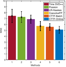
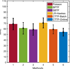
We evaluate our method (CTTF) on two real-world datasets, and we segment each into several subsets. For each subset, we use all the events up to a predefined timestamp as the training data, and the remaining events as the testing data. The hyper-parameters, including {ρ, α, β} in our method and the w in kernel κ(t) are selected using 10-fold cross validation with grid search. Using the prediction method mentioned in Sec. 4.3, we predict the number of events happening in the testing time interval and report the Mean Absolute Error (MAE) between the predicted and true number. The mean and the standard deviation of the MAEs obtained in different subsets are shown as errorbars in Fig. 3(a) and 3(b).

We consider the following methods as baselines, for comparison. In the case of 2D tensor (matrix) data, we implement four methods: classical matrix factorization TimeSVD++ [Koren, 2010], dynamic Poisson factorization [Charlin et al., 2015], low-rank regularized Hawkes process (LR-Hawkes) [Du et al., 2015], and the co-evolutionary feature process

(CoevolveFP) [Wang et al., 2016]. In the case of 3D tensor data, besides the Poisson and the CoevolveFP, we compare with Bayesian probabilistic tensor factorization (BPTF) [Xiong et al., 2010], and the scalable Bayesian nonnegative tensor factorization method (SBTF) [Hu et al., 2015].

Similar to our work, the LR-Hawkes and the CoevolveFP are point process-based methods, which estimate the number of future events by the simulation method in Sec. 4.3. The TimeSVD++ can also describe event sequences in continuous time. It estimates the number of future events directly by learned latent factors and a predefined decay function of time. For the other methods, which cannot factorize tensors in the continuous-time domain, we first reformulate original data as time series: the event sequence is discretized into several bins and the numbers of the events with different types in each bin are recorded. The training count tensor is fitted by these methods and the testing count tensor is estimated by the learned latent factors.

Additionally, in both these two cases, we implement our CTTF method by batch optimization and online optimization, respectively (CTTF-Batch and CTTF-Online). The CTTFBatch assumes that the whole training sequence obeys to a stationary point process, and we learn a single pairwise interactive point process model. The CTTF-Online relaxes the stationary assumption and updates the model online by importing small batches of training events sequentially. The testing sequence is then estimated by the model in last updating.

6.2 IPTVDataset

The IPTV dataset [Wang et al., 2016; Luo et al., 2014] contains the watching history of 7, 100 users, of 436 drama programs in 11 months, with 2, 392, 010 events, and 1, 420 binary movie features, including 1, 073 actors, 312 directors, 22 genres, 8 countries and 5 years. There are two modalities corresponding to "user" and "TV program", and each counting process N(t) counts how many viewing behaviors of a specific user-program pair happen till time t. We re-

(a) Comparisons on IPTV

Methods

(b) Comparisons on GDELT

Figure 3: Experimental results and comparisons.

duce the dimension of these features to 20 (= D) by nonnegative sparse principal component analysis [Zass and Shashua, 2007]. We can treat the counting processes as a continuoustime 2D tensor, whose elements record the numbers of modality pairs (i.e., user ID and drama ID). We segment the dataset into 47 subsets, each of which corresponds to user watching records over a contiguous span of 192 hours (8 days). For each method, the data in the first 168 hours is used to train the model and the remaining data is used to test.

Figure 3(a) visualizes the comparisons for various methods on the average and the standard deviation of MAEs. We find that the our CTTF-Online method obtains smaller MAE with smaller standard deviation, outperforming the comparison methods. In particular, the TimeSVD++ considers the influence of historical observations on current interactions among different modalities but it does not take advantages of features of events in its framework. The dynamic Poisson method only considers the transition probability between adjacent events, which cannot capture more complicated triggering patterns. The LR-Hawkes method does not consider the interactions across different modalities, considering the event sequences corresponding to different multimodal event types independently. The CoevolveFP method does not consider the interaction with each modality. The LR-Hawkes and CoevolveFP methods are inferior to the proposed CTTF because they only model one-side interactions. Moreover, the CTTF-Online is slightly better than the CTTF-Batch. In practice, the target model often may be locally-stationary rather than globally-stationary, and the testing data is likely to have more similar dynamics to its adjacent training data. The CTTF-Online updates the model online and captures its evolution over time.

6.3 Political Science Dataset

We next consider a dataset from the Global Database of Events, Location, and Tone (GDELT) [Leetaru and Schrodt, 2013]. It records the dyadic interactions between countries in the form of Country A did something to Country B at a certain time. Here, we consider 88 countries, 16 types of actions, and a time period of 2, 395 days (from years 2007 to 2013), containing 9, 825, 248 events. In particular, each event is associated with two attributes called "QuadClass" and "Coldstein", respectively. The "QuadClass" indicates that the action in the event belongs to one of the following

MAE

four classes: Verbal Cooperation, Material Cooperation, Verbal Conflict, and Material Conflict. The "Coldstein" is in the range of [-10, 10]. It represents positive (negative) events by positive (negative) values, and its amplitude indicates the infectivity of the event. Therefore, we represent these two attributes as a 25-dimensional binary feature vector for each event. There are three modalities corresponding to "political action type", "the country applying action" and "the country suffering action", and each N(t) records the number of "country-country-action type" triples up to time t. The counting processes of the interactions among the countries is formulated as a continuous-time 3D tensor. In this experiment, we segment the GDELT dataset into 39 subsets, each of which corresponds to the political events in 9 weeks (63 days). For each method, the data in the first 8 weeks is used to train the model and the remaining data is used to test.

Figure 3(b) visualizes the comparisons for the different methods, on the average and the standard deviation of MAEs. Similar to the experiments on the IPTV dataset, our CTTFOnline method is superior to the alternative approaches. In this experiment, the TimeSVD++ and the CoevolveFP are designed for the 2D case, which are unsuitable for 3D tensor data. The LR-Hawkes method treats the sequences with specific multimodal event types independently, and suffers from over-fitting, yielding an MAE that is larger than the methods. The BPTF is originally designed for the 2D case as well, but it can be easily extended to the 3D case. Similar to the Poisson method, it only considers the transitions between adjacent events, and thus cannot capture high-order relationships. The most competitive baseline of our method in this experiment is the SBFT method, which achieves comparable performance to the CTTF-Batch method. However, it is still inferior to the CTTF-Online method because it ignores the evolution of the model over time.

7 Conclusions

We propose a pairwise interactive point process model to achieve online continuous-time tensor factorization for multimodal event sequences. The learning task of the proposed model can be reformulated as a convex optimization problem, which can be solved by an online ADMM. We analyze the convergence and the computational complexity of our method, and demonstrate its feasibility and superiority on two real-world datasets. In the future, we plan to introduce the online learning strategy into the framework of maximum likelihood estimation, with the goal of achieving a better convergence rate. Additionally, the neural network-based embedding methods will be considered for the latent factors.

Acknowledgments

The work presented here was supported in part by DARPA, DOE, NIH, NSF and ONR.