
Binary Coding based Label Distribution Learning
Proceedings of the Twenty-Seventh International Joint Conference on Artificial Intelligence. Main track. Pages 2783-2789.
https://doi.org/10.24963/ijcai.2018/386
Keywords
- Machine Learning Applications: Big data ; Scalability
- Machine Learning: Machine Learning
Abstract
Label Distribution Learning (LDL) is a novel learning paradigm in machine learning, which assumes that an instance is labeled by a distribution over all labels, rather than labeled by a logic label or some logic labels. Thus, LDL can model the description degree of all possible labels to an instance. Although many LDL methods have been put forward to deal with different application tasks, most existing methods suffer from the scalability issue. In this paper, a scalable LDL framework named Binary Coding based Label Distribution Learning (BC-LDL) is proposed for large-scale LDL. The proposed framework includes two parts, i.e., binary coding and label distribution generation. In the binary coding part, the learning objective is to generate the optimal binary codes for the instances. We integrate the label distribution information of the instances into a binary coding procedure, leading to high-quality binary codes. In the label distribution generation part, given an instance, the k nearest training instances in the Hamming space are searched and the mean of the label distributions of all the neighboring instances is calculated as the predicted label distribution. Experiments on five benchmark datasets validate the superiority of BC-LDL over several state-of-the-art LDL methods.
- [Gao et al., 2017] Bin-Bin Gao, Chao Xing, Chen-Wei Xie, Jianxin Wu, and Xin Geng. Deep label distribution learn- ing with label ambiguity. IEEE Transactions on Image Processing, 26(6):2825-2838, 2017.
- [Geng and Hou, 2015] Xin Geng and Peng Hou. Pre-release prediction of crowd opinion on movies by label distribu- tion learning. In IJCAI, pages 3511-3517, 2015. IJCAI
- [Geng et al., 2013] Xin Geng, Chao Yin, and Zhi-Hua Zhou. Facial age estimation by learning from label distribution- s. IEEE Transactions on Pattern Analysis and Machine Intelligence, 35(10):2401-2412, 2013.
- [Geng, 2016] Xin Geng. Label distribution learning. IEEE Transactions on Knowledge and Data Engineering, 28(7):1734-1748, 2016.
- [Indyk and Motwani, 1998] Piotr Indyk and Rajeev Mot- wani. Approximate nearest neighbors: towards removing the curse of dimensionality. In Proceedings of the thirtieth annual ACM symposium on Theory of computing, pages 604-613. ACM, 1998.
- [Jiang and Li, 2015] Qing-Yuan Jiang and Wu-Jun Li. Scal- able graph hashing with feature transformation. In IJCAI, pages 2248-2254, 2015. IJCAI
- [Kang et al., 2016] Wang-Cheng Kang, Wu-Jun Li, and Zhi- Hua Zhou. Column sampling based discrete supervised hashing. In AAAI, pages 1230-1236, 2016.
- [Lin et al., 2013] Guosheng Lin, Chunhua Shen, David Suter, and Anton Van Den Hengel. A general two-step approach to learning-based hashing. In Proceedings of the IEEE International Conference on Computer Vision, pages 2552-2559, 2013.
- [Lin et al., 2014] Guosheng Lin, Chunhua Shen, Qinfeng Shi, Anton Van den Hengel, and David Suter. Fast su- pervised hashing with decision trees for high-dimensional data. In Proceedings of the IEEE Conference on Computer Vision and Pattern Recognition, pages 1963-1970, 2014.
- [Liu et al., 2012] Wei Liu, Jun Wang, Rongrong Ji, Yu-Gang Jiang, and Shih-Fu Chang. Supervised hashing with ker- nels. In Computer Vision and Pattern Recognition (CVPR), 2012 IEEE Conference on, pages 2074-2081. IEEE, 2012.
- [Quan and Ren, 2010] Changqin Quan and Fuji Ren. Sen- tence emotion analysis and recognition based on emotion words using ren-cecps. International Journal of Advanced Intelligence, 2(1):105-117, 2010.
- [Ricanek and Tesafaye, 2006] Karl Ricanek and Tamirat Tesafaye. Morph: A longitudinal image database of nor- mal adult age-progression. In Automatic Face and Gesture Recognition, 2006. FGR 2006. 7th International Confer- ence on, pages 341-345. IEEE, 2006.
- [Sarwar et al., 2001] Badrul Sarwar, George Karypis, Joseph Konstan, and John Riedl. Item-based collaborative filter- ing recommendation algorithms. In Proceedings of the 10th international conference on World Wide Web, pages 285-295. ACM, 2001.
- [Shen et al., 2015] Fumin Shen, Chunhua Shen, Wei Liu, and Heng Tao Shen. Supervised discrete hashing. In Pro- ceedings of the IEEE Conference on Computer Vision and Pattern Recognition, pages 37-45, 2015.
- [Simonyan and Zisserman, 2014] Karen Simonyan and An- drew Zisserman. Very deep convolutional networks for large-scale image recognition. arXiv preprint arX- iv:1409.1556, 2014.
- [Wang et al., 2010] Jun Wang, Sanjiv Kumar, and Shih-Fu Chang. Sequential projection learning for hashing with compact codes. In Proceedings of the 27th international conference on machine learning (ICML-10), pages 1127- 1134, 2010.
- [Wang et al., 2012] Jun Wang, Sanjiv Kumar, and Shih-Fu Chang. Semi-supervised hashing for large-scale search. IEEE Transactions on Pattern Analysis and Machine In- telligence, 34:2393-2406, 2012.
- [Wang et al., 2016] Xiaojuan Wang, Ting Zhang, Guo-Jun Qi, Jinhui Tang, and Jingdong Wang. Supervised quan- tization for similarity search. In Proceedings of the IEEE Conference on Computer Vision and Pattern Recognition, pages 2018-2026, 2016.
- [Weiss et al., 2009] Yair Weiss, Antonio Torralba, and Rob Fergus. Spectral hashing. In Advances in neural informa- tion processing systems, pages 1753-1760, 2009.
- [Xing et al., 2016] Chao Xing, Xin Geng, and Hui Xue. Lo- gistic boosting regression for label distribution learning. In Proceedings of the IEEE Conference on Computer Vision and Pattern Recognition, pages 4489-4497, 2016.
- [Yang et al., 2016] Xu Yang, Xin Geng, and Deyu Zhou. S- parsity conditional energy label distribution learning for age estimation. In IJCAI, pages 2259-2265, 2016. IJCAI
- [Yang et al., 2017] jufeng Yang, ming Sun, and xiaoxiao Sun. Learning visual sentiment distributions via augment- ed conditional probability neural network. In AAAI, pages 224-230, 2017.
- [Zhang and Li, 2014] Dongqing Zhang and Wu-Jun Li. Large-scale supervised multimodal hashing with seman- tic correlation maximization. In AAAI, volume 1, page 7, 2014.
- [Zhou et al., 2015] Ying Zhou, Hui Xue, and Xin Geng. E- motion distribution recognition from facial expressions. In Proceedings of the 23rd ACM international conference on Multimedia, pages 1247-1250. ACM, 2015.
- [Zhou et al., 2016] Deyu Zhou, Xuan Zhang, Yin Zhou, Quan Zhao, and Xin Geng. Emotion distribution learning from texts. In EMNLP, pages 638-647, 2016.
- [Zhu and Gao, 2017] Hao Zhu and Sheng-Hua Gao. Locality-constrained deep supervised hashing for image retrieval. In IJCAI, pages 3567-3573, 2017. IJCAI
References were extracted automatically from the PDF and may contain errors.
Full text extracted automatically from the PDF; figures, tables and equations may differ. The PDF is the version of record.
1 Introduction
Learning with ambiguity plays a fundamental role in many areas including machine learning, computer vision, data mining and so on. Although different varieties of learning paradigms have been proposed for learning with ambiguity, label distribution learning (LDL) has become one of the latest approaches to this goal because it can perform better than other paradigms in some real applications [Geng et al., 2013; Zhou et al., 2016; Xing et al., 2016; Yang et al., 2016; Gao et al., 2017]. Generally speaking, LDL assumes that an instance x is labeled by a real number dyx to every possible label y, representing the degree to which the corresponding y describes x. Thus, dyx is named the description degree of y to the instance x. The vector consisting of the description degrees of all the labels is called label distribution because it is similar to probability distribution. Label distribution can not only model the ambiguity of "what describes the instance", but also deal with the more general ambiguity of "how to describe the instance" [Xing et al., 2016]. Without loss of generality, LDL assumes that dyx ∈ [0, 1] and ∑y dyx = 1. Different from other learning paradigms, single-label learning (SLL) and multi-label learning (MLL) for example, the main purpose of LDL is to learn a group of mapping functions from the instance to its label distribution.
∗Corresponding author.
In recent years, a collection of LDL algorithms have been proposed. The representative methods include IISLDL [Geng et al., 2013], conditional probability neural network (CPNN) [Geng et al., 2013], label distribution support vector regressor (LDSVR) [Geng and Hou, 2015], BFGSLDL [Geng, 2016], PT-Bayes [Geng, 2016], PT-SVM [Geng, 2016], AA-BP [Geng, 2016], LDLogitBoost [Xing et al., 2016], AOSO-LDLogitBoost [Xing et al., 2016], sparsity conditional energy label distribution learning (SCE-LDL) [Yang et al., 2016], deep label distribution learning (DLDL) [Gao et al., 2017] and so on. However, most of them suffer from one key limitation: as the size of training set increases, the training time grows rapidly.
To avoid the high training time consumption, Geng (2016) proposed a method known as AA-kNN, which is an adaptation algorithm of k-Nearest Neighbor (k-NN) to solve the LDL problem. Compared with other LDL algorithms, the advantage of AA-kNN is that it does not need a training process. However, AA-kNN suffers from two drawbacks. Firstly, its performance heavily depends on the quality of the original features it uses, which are usually extracted in an unsupervised way. Thus, when the high quality features cannot be obtained, it may lead to poor performance. Secondly, when the size of dataset is large and the dimension of real-valued feature is high, the testing phase (linear search) will cost a great deal of time. Therefore, like most of other LDL methods, AA-kNN is not applicable to large-scale LDL.
To address the above-mentioned problems, we employ the binary coding/hashing techniques to tackle the task of largescale LDL, which is widely used for approximate nearest neighbor (ANN) search [Indyk and Motwani, 1998]. The purpose of hashing is to transform high-dimensional original features into compact binary codes. Since the representations of instances are compressed as short binary codes, the time and memory cost of searching process can be significantly reduced.
Existing hashing methods can be roughly categorized into two groups, i.e., unsupervised hashing and supervised (including semi-supervised) hashing. As label information is useful for generating more discriminative hash codes, supervised hashing methods can often achieve better performance. Existing representative supervised hashing algorithms include sequential projection learning for hashing (SPLH) [Wang et al., 2010], supervised hashing with kernels (KSH) [Liu et al., 2012], two-step hashing (TSH) [Lin et al., 2013], FastHash [Lin et al., 2014], supervised discrete hashing (SDH) [Shen et al., 2015], column sampling based discrete supervised hashing (COSDISH) [Kang et al., 2016], supervised quantization (SQ) [Wang et al., 2016]. However, most existing supervised hashing methods are developed for the instances labeled by a logic label or some logic labels. They cannot directly integrate the label distribution information into the binary coding procedure. Thus, it is not much appropriate to extend most existing supervised hashing methods to deal with LDL problem.
It is worth noting that Jiang and Li (2015) put forward the scalable graph hashing (SGH) method, which exploits a feature transformation technique to approximate the whole graph. The time complexity of SGH is O(n), because the pairwise similarity graph matrix is avoided explicitly computing. Although the performance of SGH is promising, the binary codes are learned in an unsupervised manner and the supervised information is not fully considered.
Inspired by AA-kNN and SGH, a scalable LDL framework, termed Binary Coding based Label Distribution Learning (BC-LDL), is put forward to solve the large-scale LDL problem. The main contributions of this paper are briefly listed as follows:
- We propose a novel supervised binary coding method for the instances labeled by the label distributions. Because we consider the correlations between the instances based on their semantic label distributions, highly discriminative binary codes can be generated by the proposed method.
- Combining binary coding and ANN search together, we further propose a scalable LDL framework for efficiently solving the large-scale LDL problem. Compared with other NN-based LDL methods (e.g., AA-kNN), the time cost of the testing phase can be greatly reduced, because the similarity of two instances can be rapidly measured by calculating the Hamming distance between two groups of binary codes via XOR operations.
- Experimental results on five real-world datasets demonstrate that the proposed BC-LDL is competitive with the state-of-the-art LDL methods.
The rest of this paper is organized as follows. Firstly, the details of the proposed BC-LDL method are presented. Secondly, the experimental results on five public datasets are reported. Finally, the conclusion is given.
2 BC-LDL
2.1 ProblemFormulation
Let X = [x1; x2; · · · ; xn] ∈ Rn×m denote the input space, Y = {y1, y2, · · · , yc} denote the complete set of labels, and dyx denote the description degree of the label y ∈ Y to the instance x ∈ X. c is the number of the labels. dyx needs to satisfy two constrains, i.e., dyx ∈ [0, 1] and ∑y dyx = 1. Without loss of generality, let X be normalized to have zero mean. Suppose that we have a training set Z = {(x1, d1), (x2, d2, ), · · · , (xn, dn)}, where n is the number of instances, xi ∈ R1×m, and di = [dy1 xi , dy2 xi , · · · , dyc xi ] is the corresponding label distribution of the instance xi.
Different from most existing LDL methods, BC-LDL does not learn a group of mapping functions from x ∈ R1×m to d ∈ R1×c directly. BC-LDL aims at learning a group of binary coding functions based on the training set Z, i.e., h(x): R1×m -→ {-1, 1}1×l , where l is the length of binary codes. Then, the ANN search strategy is employed to generate the label distributions for the testing instances. In this paper, h(x) is defined as follows:
where sign(·) denotes the element-wise sign function, which returns 1 if the element is a positive number and returns -1 otherwise. W ∈ Rm×l is the mapping matrix, and e ∈ R1×l is the bias vector.
2.2 Binary Coding
Similar to some existing supervised hashing methods [Liu et al., 2012; Zhang and Li, 2014; Lin et al., 2014; Kang et al., 2016], we expect to approximate the similarity matrix S by the generated binary codes of training instances. Thus, we have the following objective function:
where B is the binary code matrix, and || · ||F denotes the Frobenius norm.
The analytical form of the objective function is:
2.3 SimilarityMatrix Construction
As aforementioned, each instance is labeled by a distribution over all labels in LDL, rather than labeled by a logic label or some logic labels. Thus, we cannot construct the similarity matrix by modeling the label consistency between instances, which is used in many supervised hashing algorithms [Wang et al., 2010; Liu et al., 2012; Lin et al., 2013; Zhu and Gao, 2017]. Furthermore, we think a real number within the range of -1 and 1 is more appropriate to represent the similarity between two instances than a logic number (i.e., -1 or 1) in LDL, because the former is more discriminative.
Based on the above considerations, we adopt the adjusted cosine similarity (ACS) metric [Sarwar et al., 2001] to construct the similarity matrix S ∈ [-1, 1]n×n . Given an instance pair (xi, xj) from the training set, the semantic affinity of this instance pair is defined as follows:
where "·" denotes the inner product of two vectors, || · ||2 denotes the L2 norm of the vector, µ is the mean of the label distributions of all the training instances, andDi∗ = di-µ ||di-µ||2 .
Then we can obtain the similarity matrix S = DDT . In fact, if we construct the similarity matrix directly, it will lead to the high time complexity and memory requirement. Therefore, we need to avoid the construction of similarity matrix S in our algorithm. In the following subsection, we will describe how to achieve it in detail.
2.4 Optimization
There is a matrix variable W and a vector variable e in our original objective function. Actually, if we denote X = [X, 1n] and W = [W; e], we can omit e and obtain the following form with only a matrix variable W :
The objective function in (5) is hard to be solved directly due to the existence of sign function. A common solution is to adopt the spectral relaxation trick [Weiss et al., 2009] and impose orthogonality constraints, i.e., W T XT XW = In. Here, In denotes a n × n identity matrix. Then, the optimization problem can be easily transferred into a generalized eigenvalue problem. However, it has been verified that non-orthogonal mapping functions can perform better than orthogonal ones in some real applications [Wang et al., 2010; Zhang and Li, 2014]. Thus, we apply a sequential learning strategy to learn the binary coding functions without imposing orthogonality constraints [Liu et al., 2012; Zhang and Li, 2014; Jiang and Li, 2015].
Suppose that we have learned the mapping functions w1,w2, · · · ,wt-1, we need to learn the next mapping function wt. We define a residual matrix Rt as follows:
Following the objective function in (5), the corresponding optimization problem to learn wt can be defined as:
The main idea of this sequential learning strategy is to reconstruct the similarity matrix by the learned binary codes and learn a new mapping function to correct the errors made by the previous ones [Wang et al., 2012; Zhang and Li, 2014].
By some algebraic calculation, we further rewrite the objective function in (7) as:
where At = sign(Xwt), and tr(·) denotes the trace operator.
Thus, the objective function in (7) can be reformulated as:
The objective function in (9) is still hard to be solved directly due to the existence of sign function. Here we use a widely-adopted approximate representation of sign function [Wang et al., 2010; 2012], i.e., sign(a) ≈ a, to handle it. We rewrite it as follows:max
where the orthogonality constraint is set to avoid the trivial solution.
It is easy to see that the optimization problem in (10) is an eigensystem problem and the eigenvector of XT RtX corresponding to its largest eigenvalue (λmax) is the approximate solution wt:
We define Gt = XT RtX, then we can obtain:
where Ai = sign(Xwi). According to the equation (12), we can find that the construction of similarity matrix S is avoided during the optimization procedure. It considerably boosts the scalability of our algorithm.
2.5 Label Distribution Generation
Our BC-LDL adopts a two-step strategy to learn the label distributions for the testing instances. In the first step, BC-LDL generates the binary codes for a new testing instance ˜x according to the equation (1): ˜b = sign(˜xW + e). In the second step, ANN search is conducted to find the k nearest training instances represented by binary codes in the Hamming space. Then, the mean of the label distributions of all the searched training instances is calculated as the learned label distribution.
Algorithm 1 BC-LDL: Train Algorithm
- 1: Input: Feature matrix X; Adjusted label distributions matrix D; Code length l.
- 2: Output: Projection matrixW; Bias vector e.
- 3: X ← [X, 1n].
- 4: G0 ← (XT D)(XT D)T .
- 5: G1 ← lG0.
- 6: for t = 1, · · · , l do
- 7: Solve the following eigensystem problem Gtwt = λmaxwt;
- 8: Obtain the mapping vector wt corresponding to the largest eigenvalue λmax;
- 9: Z ← [XT sign(Xwt)][XT sign(Xwt)]T ;
- 10: Gt+1 ←Gt -Z;
- 11: end for
- 12: W ← [w1,w2, · · · ,wl].
- 13: W ←W(1 : end-1, :); e ←W(end, :).
Algorithm 2 BC-LDL: Test Algorithm
- 1: Input: Test instance ˜x; No. of nearest neighbors k.
- 2: Output: Label distribution ˜ d.
- 3: ˜b ← sign(˜xW +e).
- 4: Nk ← the k nearest neighbors of ˜b in the Hamming space.
- 5: ˜ d ← the mean of the label distributions of the instances ∈ Nk.
2.6 Summary and Analysis
We summarize the proposed BC-LDL method in Algorithm 1 and Algorithm 2.
In the training phase, the time complexity of BC-LDL includes two aspects, i.e., the initialization procedure and the sequential learning procedure. Firstly, initialization of G0 will cost O(cn(m+1)+c(m+1)2 ). Secondly, the time cost of the sequential learning procedure is O(l((m+1)3 +(m+ 1)n + (m+ 1)2 )). The training time complexity of BC-LDL is linear to n, because c, l,m is usually much less than n.
In the testing phase, the time cost of generating the binary codes for a testing instance is O(lm) and searching the k nearest training instances is O(kn). Hence, the testing time complexity is O(lm+ kn) in total.
We can see that when the size of training set is large, the testing phase will cost much time. An effective solution for this problem is that we can construct a hash table to store the mean of the label distributions of these training instances with the same binary codes. Then, the mean is used as the predicted label distribution for a testing instance that have the same binary codes. The time cost of constructing a hash table is O(2ln) and predicting the label distribution for a testing instance will cost O(lm+ l2l ). We set l = 8 in this paper, and thus 2l ≪ n. Altogether, the training time complexity is still O(n). This method is named as BCTable.
3 Experiment
In this section, we evaluate the proposed algorithms on five different datasets: s-BU 3DFE (scores-Binghamton University 3D Facial Expression) [Zhou et al., 2015], COPM (Crowd Opinion Prediction on Movies) [Geng and Hou, 2015], Twitter LDL [Yang et al., 2017], Ren-CECps [Quan and Ren,
| Dataset | #instance | #dim | #label |
|---|---|---|---|
| s-BU 3DFE | 2,500 | 243 | 6 |
| COPM | 7,755 | 1,869 | 5 |
| Twitter LDL | 10,045 | 200 | 8 |
| Ren-CECps | 35,096 | 100 | 8 |
| MORPH | 55,132 | 200 | 60 |
2010] and MORPH [Ricanek and Tesafaye, 2006]. Due to the space limitation, here we only present the brief statistics of these evaluated datasets in Table 1. All the experiments are carried on a PC with Intel (R) Core (TM) CPU i5-6300@2.30GHz and 12GB RAM.
3.1 Experimental Settings
To validate the proposed methods, we comprehensively compare them with several baselines. These algorithms include four specialized algorithms IIS-LDL, BFGS-LDL, CPNN, LDSVR, and one adaptation algorithm AA-kNN.
As suggested in [Geng, 2016], six measures are employed to evaluate the accuracy performance of all the methods. Among them, Chebyshev, Clark, Canberra, Kullback-Leibler (K-L), measure the distance between two distributions, thus they are the smaller the better. Cosine and Intersection are used to measure the similarity between two distributions, so they are the larger the better.
The parameters of all the methods used in the experiments are carefully tuned and the best results of baseline methods are reported. On s-BU 3DFE, k in BC-LDL is set to 20 and code length is set to 32 bits. The maximum iteration steps in BFGS-LDL is 300 and IIS-LDL is 100. k for AA-kNN is set to 20. On COPM, k in BC-LDL is 30 and code length is 128 bits. The maximum iteration steps in BFGS-LDL is 100 and IIS-LDL is 20. k in AA-kNN is 10. On Twitter LDL, k in BC-LDL is set to 10 and code length is 256 bits. The maximum iteration steps in BFGS-LDL is 300 and IIS-LDL is 50. k in AA-kNN is 10. On Ren-CECps, k in BC-LDL is 20 and code length is set to 64 bits. The maximum iteration steps in BFGS-LDL is 200 and IIS-LDL is 100. k in AAkNN is set to 20. On MORPH, k in BC-LDL is set to 50 and code length is 256 bits. The maximum iteration steps in BFGS-LDL is 100 and IIS-LDL is 20. k in AA-kNN is set to 10. On the five datasets, the insensitivity parameter ε of LDSVR is set to 0.1 and the number of hidden-layer neurons of CPNN is set to 50.
All the results are averaged over 10-fold cross validation in terms of both accuracy and time cost.
3.2 Experimental Results
Table 2-6 report the results of our methods and other baselines on the five evaluated datasets. When we evaluate the performance of a LDL algorithm, its accuracy performance and efficiency performance are equally important. Hence, three different rank metrics are adopted to evaluate the performance of all the algorithms in our experiments, i.e., Accuracy Rank (Acc. Rank), Time Rank and Average Rank (Avg. Rank), which can reflect the accuracy, efficiency and comprehensive performance of these algorithms, respectively. 1 Furthermore, the ranks of six measure values are also given in the parentheses right after the corresponding measure values, and the average value of these six ranks is denoted as Acc. Rank. Note that Avg. Rank of an algorithm is the average value between its Acc. Rank and Time Rank.
| Method | Accuracy | Time Cost(s) | Avg. Rank | ||||||||
|---|---|---|---|---|---|---|---|---|---|---|---|
| Cheb↓ | Clark↓ | Canber↓ | K-L↓ | Cosine↑ | Intersec↑ | Acc. Rank | Train | Test | Sum(Time Rank) | ||
| BC-LDL | 0.102(1) | 0.323(1) | 0.666(1) | 0.054(1) | 0.946(1) | 0.879(1) | 1.00 | 0.128 | 0.020 | 0.148(2) | 1.50 |
| BCTable | 0.117(4) | 0.364(4) | 0.763(4) | 0.067(5) | 0.934(5) | 0.861(4) | 4.33 | 0.045 | 0.002 | 0.047(1) | 2.67 |
| BFGS-LDL | 0.105(2) | 0.355(3) | 0.742(3) | 0.056(3) | 0.945(2) | 0.869(3) | 2.67 | 90.86 | 0.004 | 90.86(6) | 4.34 |
| IIS-LDL | 0.121(5) | 0.376(5) | 0.805(5) | 0.065(4) | 0.936(4) | 0.856(5) | 4.67 | 366.5 | 0.001 | 366.5(7) | 5.84 |
| CPNN | 0.106(3) | 0.346(2) | 0.729(2) | 0.055(2) | 0.944(3) | 0.870(2) | 2.33 | 38.89 | 0.022 | 38.91(5) | 3.67 |
| LDSVR | 0.126(7) | 0.383(6) | 0.826(7) | 0.072(6) | 0.929(6) | 0.852(6) | 6.33 | 1.304 | 0.025 | 1.329(4) | 5.17 |
| AA-kNN | 0.125(6) | 0.388(7) | 0.822(6) | 0.073(7) | 0.928(7) | 0.852(6) | 6.50 | 0 | 1.283 | 1.283(3) | 4.75 |
| Method | Accuracy | Time Cost(s) | Avg. Rank | ||||||||
|---|---|---|---|---|---|---|---|---|---|---|---|
| Cheb↓ | Clark↓ | Canber↓ | K-L↓ | Cosine↑ | Intersec↑ | Acc. Rank | Train | Test | Sum(Time Rank) | ||
| BC-LDL | 0.115(2) | 0.518(2) | 0.992(2) | 0.100(2) | 0.934(2) | 0.836(2) | 2.00 | 8.633 | 0.240 | 8.873(2) | 2.00 |
| BCTable | 0.118(3) | 0.532(4) | 1.017(4) | 0.103(3) | 0.932(3) | 0.832(4) | 3.50 | 0.705 | 0.007 | 0.712(1) | 2.25 |
| BFGS-LDL | 0.119(4) | 0.522(3) | 1.003(3) | 0.104(4) | 0.931(4) | 0.833(3) | 3.50 | 144.8 | 0.006 | 144.8(5) | 4.25 |
| IIS-LDL | 0.138(6) | 0.561(6) | 1.078(6) | 0.122(6) | 0.917(6) | 0.814(6) | 6.00 | 611.4 | 0.004 | 611.4(7) | 6.50 |
| CPNN | 0.144(7) | 0.615(7) | 1.188(7) | 0.157(7) | 0.899(7) | 0.798(7) | 7.00 | 360.7 | 0.154 | 360.9(6) | 6.50 |
| LDSVR | 0.112(1) | 0.499(1) | 0.966(1) | 0.097(1) | 0.936(1) | 0.840(1) | 1.00 | 25.37 | 0.505 | 25.88(3) | 2.00 |
| AA-kNN | 0.121(5) | 0.545(5) | 1.041(5) | 0.108(5) | 0.929(5) | 0.827(5) | 5.00 | 0 | 124.9 | 124.9(4) | 4.50 |
| Method | Accuracy | Time Cost(s) | Avg. Rank | ||||||||
|---|---|---|---|---|---|---|---|---|---|---|---|
| Cheb↓ | Clark↓ | Canber↓ | K-L↓ | Cosine↑ | Intersec↑ | Acc. Rank | Train | Test | Sum(Time Rank) | ||
| BC-LDL | 0.266(2) | 2.080(1) | 4.841(1) | 0.469(2) | 0.846(2) | 0.669(2) | 1.67 | 1.191 | 0.391 | 1.582(2) | 1.84 |
| BCTable | 0.282(4) | 2.396(3) | 6.210(3) | 0.584(4) | 0.836(4) | 0.643(4) | 3.67 | 0.106 | 0.008 | 0.114(1) | 2.34 |
| BFGS-LDL | 0.460(6) | 2.410(5) | 6.290(5) | 1.142(6) | 0.637(6) | 0.433(6) | 5.67 | 48.73 | 0.004 | 48.73(4) | 4.84 |
| IIS-LDL | 0.500(7) | 2.400(4) | 6.249(4) | 1.172(7) | 0.589(7) | 0.387(7) | 6.00 | 264.4 | 0.002 | 264.4(7) | 6.50 |
| CPNN | 0.306(5) | 2.447(7) | 6.421(7) | 0.754(5) | 0.799(5) | 0.621(5) | 5.67 | 163.3 | 0.106 | 163.4(5) | 5.34 |
| LDSVR | 0.267(3) | 2.420(6) | 6.338(6) | 0.553(3) | 0.840(3) | 0.665(3) | 4.00 | 245.4 | 0.272 | 245.7(6) | 5.00 |
| AA-kNN | 0.261(1) | 2.090(2) | 4.878(2) | 0.465(1) | 0.854(1) | 0.674(1) | 1.33 | 0 | 16.26 | 16.26(3) | 2.17 |
| Method | Accuracy | Time Cost(s) | Avg. Rank | ||||||||
|---|---|---|---|---|---|---|---|---|---|---|---|
| Cheb↓ | Clark↓ | Canber↓ | K-L↓ | Cosine↑ | Intersec↑ | Acc. Rank | Train | Test | Sum(Time Rank) | ||
| BC-LDL | 0.566(1) | 2.329(1) | 5.773(1) | 1.229(1) | 0.569(1) | 0.368(1) | 1.00 | 0.327 | 2.056 | 2.383(2) | 1.50 |
| BCTable | 0.600(3) | 2.639(3) | 7.261(3) | 1.422(3) | 0.550(2) | 0.318(3) | 2.83 | 0.217 | 0.022 | 0.239(1) | 1.92 |
| BFGS-LDL | 0.604(4) | 2.649(5) | 7.319(4) | 1.499(5) | 0.546(3) | 0.304(4) | 4.17 | 202.1 | 0.004 | 202.1(4) | 4.09 |
| IIS-LDL | 0.625(6) | 2.654(6) | 7.357(6) | 1.564(6) | 0.519(6) | 0.272(6) | 6.00 | 424.7 | 0.003 | 424.7(5) | 5.50 |
| CPNN | 0.620(5) | 2.648(4) | 7.320(5) | 1.476(4) | 0.534(5) | 0.287(5) | 4.67 | 484.7 | 0.270 | 485.0(6) | 5.34 |
| LDSVR1 | - | - | - | - | - | - | - | - | - | - | - |
| AA-kNN | 0.593(2) | 2.393(2) | 6.073(2) | 1.342(2) | 0.536(4) | 0.328(2) | 2.33 | 0 | 157.2 | 157.2(3) | 2.67 |
| Method | Accuracy | Time Cost(s) | Avg. Rank | ||||||||
|---|---|---|---|---|---|---|---|---|---|---|---|
| Cheb↓ | Clark↓ | Canber↓ | K-L↓ | Cosine↑ | Intersec↑ | Acc. Rank | Train | Test | Sum(Time Rank) | ||
| BC-LDL | 0.081(2) | 6.777(2) | 49.34(2) | 0.716(2) | 0.719(2) | 0.563(3) | 2.17 | 5.644 | 12.29 | 17.93(2) | 2.09 |
| BCTable | 0.086(4) | 6.826(5) | 49.92(5) | 0.748(3) | 0.700(4) | 0.533(4) | 4.17 | 0.626 | 0.045 | 0.671(1) | 2.58 |
| BFGS-LDL | 0.087(5) | 6.812(4) | 49.81(4) | 0.897(5) | 0.684(5) | 0.511(5) | 4.67 | 223.9 | 0.012 | 223.9(3) | 3.83 |
| IIS-LDL | 0.110(6) | 6.892(6) | 51.03(6) | 1.119(6) | 0.573(6) | 0.367(6) | 6.00 | 1379 | 0.007 | 1379(5) | 5.50 |
| CPNN | 0.083(3) | 6.802(3) | 49.59(3) | 0.654(1) | 0.727(1) | 0.569(2) | 2.17 | 2804 | 4.082 | 2808(6) | 4.09 |
| LDSVR | - | - | - | - | - | - | - | - | - | - | - |
| AA-kNN | 0.076(1) | 6.246(1) | 45.10(1) | 0.872(4) | 0.712(3) | 0.582(1) | 1.83 | 0 | 541.6 | 541.6(4) | 2.92 |
1 We don't report the experimental results of LDSVR because it would cause out of memory issue
From Table 2-6, we can find that BC-LDL achieves the best accuracy performance on two datasets (i.e., s-BU 3DFE and Ren-CECps), and achieves the second best performance on other datasets. Compared with other baselines, BC-LDL and BCTable can achieve better efficiency performance on the five evaluated datasets. Moreover, BC-LDL achieves the best comprehensive performance on the five datasets. The comprehensive performance of BC-LDL on the five evaluated datasets demonstrates its effectiveness and efficiency.
| Dataset | Baseline Method | Time Ratio | |
|---|---|---|---|
| BC-LDL | BCTable | ||
| s-BU 3DFE | AA-kNN | 8.669 | 27.30 |
| COPM | LDSVR | 2.917 | 36.35 |
| Twitter LDL | AA-kNN | 10.28 | 142.6 |
| Ren-CECps | AA-kNN | 65.97 | 657.7 |
| MORPH | BFGS-LDL | 12.49 | 333.7 |
The experimental results on s-BU 3DFE are reported in Table 2. We can see that our BC-LDL method outperforms other baseline methods, which demonstrates its superiority. Table 3 reports the experimental results on COPM. Here, we have a different observation: LDSVR achieves the better accuracy performance than BC-LDL. A reasonable explanation is that the application of the kernel trick makes LDSVR solve the LDL problem with the high-dimension features more effectively. Table 4 reports the experimental results on TwitterLDL. We can find that AA-kNN achieves the best accuracy performance. The desirable results of AA-kNN can be attributed to the high-quality original features, which are extracted by VGGNet [Simonyan and Zisserman, 2014]. Table 5 reports the experimental results on Ren-CECps. Once again, BC-LDL yields better experimental results than other baseline algorithms. Furthermore, it is worth noting that the total time consumption of BCTable is least and its results are comparable to most LDL methods. The experimental results on MORPH are reported in Table 6. Although AA-kNN achieves the better accuracy performance, its time consumption of testing phase is much more than that of our methods.
To further demonstrate the efficiency of our algorithms, we also report the time ratio of the fastest compared method to our methods. The results are reported in Table 7. We can find that our algorithms are much faster than other baseline algorithms, especially on the large-scale datasets (i.e., RenCECps and MORPH).
3.3 Analysis on Binary Code Length
In this part, we study the evaluation results variation with respect to different code lengths on the five evaluated datasets. The code length is set to {16, 32, · · · , 256} in actual experiments. Due to the space limitation, we only present the K-L and Intersection results. The results of other measures are similar. The evaluation results are reported in Figure 1-2. We have two observations. Firstly, longer binary codes can lead to better results on the medium-scale dataset (i.e., Twitter LDL) and the large-scale datasets (i.e., Ren-CECps and MORPH). However, when the code length exceeds 128 bits, the performance of BC-LDL tends to converge. It proves that BC-LDL can achieve acceptable results with reasonably short binary codes, that is crucial in large-scale LDL. Secondly, as the code length increases, the performance improvement on s-BU 3DFE and COPM is not significant. When the code length exceeds 64 bits, the performance of BC-LDL
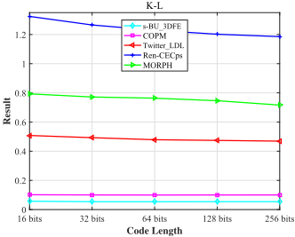
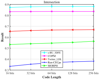
even degrades to some extent. A possible reason for this phenomenon is that the size of these two datasets is small, and thus they cannot provide more useful information for longer binary codes.
4 Conclusion
In this paper, we have proposed a scalable LDL algorithm called BC-LDL, for dealing with the large-scale LDL problem. In BC-LDL, the label distribution information is integrated into the binary coding procedure for generating highquality binary codes. Moreover, ANN search is conducted to find the training instances that have binary codes with a small Hamming distance from a testing instance, which can be efficiently computed via XOR operations. Then, the mean of the label distributions of all the neighboring instances is calculated as the predicted label distribution. Experimental results on five real-world datasets have demonstrated that BC-LDL is competitive with several state-of-the-art LDL methods.
Acknowledgments
This research was supported by the National Key Research & Development Plan of China (No. 2017YFB1002801), the National Science Foundation of China (61622203), the Jiangsu Natural Science Funds for Distinguished Young Scholar
(BK20140022), the Collaborative Innovation Center of Novel Software Technology and Industrialization, and the Collaborative Innovation Center of Wireless Communications Technology.
@inproceedings{ijcai2018p386,
  title     = {Binary Coding based Label Distribution Learning},
  author    = {Wang, Ke and Geng, Xin},
  booktitle = {Proceedings of the Twenty-Seventh International Joint Conference on
               Artificial Intelligence, {IJCAI-18}},
  publisher = {International Joint Conferences on Artificial Intelligence Organization},
  editor    = {Jérôme Lang},
  pages     = {2783--2789},
  year      = {2018},
  month     = {7},
  note      = {Main track},
  doi       = {10.24963/ijcai.2018/386},
  url       = {https://doi.org/10.24963/ijcai.2018/386},
}
TY - CPAPER TI - Binary Coding based Label Distribution Learning AU - Wang, Ke AU - Geng, Xin T2 - Proceedings of the Twenty-Seventh International Joint Conference on Artificial Intelligence, IJCAI-18 PB - International Joint Conferences on Artificial Intelligence Organization PY - 2018 SP - 2783 EP - 2789 DO - 10.24963/ijcai.2018/386 UR - https://doi.org/10.24963/ijcai.2018/386 ER -Copied
Machine-readable versions of this paper, for tools and AI agents:





